Global Mean Surface Temperature: Early 20th Century Warming Period – Models versus Models & Models versus Data

This is a long post: 3500+ words and 22 illustrations. Regardless, heretics of the church of human-induced global warming who frequent this blog should enjoy it.  Additionally, I’ve uncovered something about the climate models stored in the CMIP5 archive that I hadn’t heard mentioned or seen presented before.  It amazed even me, and I know how poorly these climate models perform.  It’s yet another level of inconsistency between models, and it’s something very basic. It should help put to rest the laughable argument that climate models are based on well-documented physical processes.

INTRODUCTION

After isolating 4 climate model ensemble members with specific characteristics (explained later in this introduction), this post presents (1) observed and climate model-simulated global mean sea surface temperatures, and (2) observed and climate model-simulated global mean land near-surface air temperatures, all during the 30-year period with the highest observed warming rate before the year 1950.  The climate model outputs being presented are those stored in the Coupled Model Intercomparison Project Phase 5 (CMIP5) archives, which were used by the Intergovernmental Panel on Climate Change (IPCC) for their 5^th Assessment Report (AR5).  Specifically, the ensemble member outputs being presented are those with historic forcings through 2005 and RCP8.5 (worst-case scenario) forcings thereafter. In other words, the ensemble members being presented during this early warming period are being driven with historic forcings, and they are from the simulations that later include the RCP8.5 forcings.

First, we’ll identify the 30-year period with the highest observed warming rate before 1950.

For climate model outputs, after presenting the multi-model mean, I first present the outputs of all 81 ensemble members (individual climate model simulations) to give you an idea of the lack of agreement among the ensemble members during the identified early warming period. Then we’ll isolate (1) the ensemble members with the highest and lowest global mean surface temperatures during that early warming period and (2) the ensemble members with the highest and lowest trends in global mean surface temperatures during that period. Those four model-ensemble members will be used for the model-data comparisons described above; i.e. global sea surface temperatures and, separately, global land near-surface air temperatures.

Last, I compare modeled global sea surface temperatures with modeled marine air temperatures and list the temperature difference for each of the ensemble members presented in this post. Would it amaze you to discover the temperature difference between modeled global sea surface temperatures and marine air temperatures is not consistent?  It amazed me.

Those readers who are not aware of how poorly climate models simulate the primary metric of climate change—global mean surface temperature—will likely be surprised by these results.

Note: I’m presenting four different metrics in this post. To make it easier for readers, I’ve added an additional identifier to the illustrations. In them, immediately above the left-hand corner of each graph, I identify (underlined in parentheses) whether the graph is presenting data or climate model outputs for (Land+Ocean) surfaces, (Ocean Only) surfaces, or (Land Only) surfaces.  [End note.]

THE CHOSEN 30-YEAR PERIOD

Figure 1 presents a model-data comparison that shows the 360-month (30-year) trends in observed and climate-model-simulated global mean land+ocean surface temperatures. It may look familiar to many of you. I used to present the same graph (without most of the notes) in my monthly Global Surface Temperature and Lower Troposphere Temperature Updates, cross posts at WattsUpWithThat are here. As noted at the bottom of Figure 1, The Period Ending about 1945 Has The Highest Observed Warming Rate before 1950. The Data Trend Is More Than 3 Times Higher Than the Trend for the Climate Model Hindcasts for that Period!

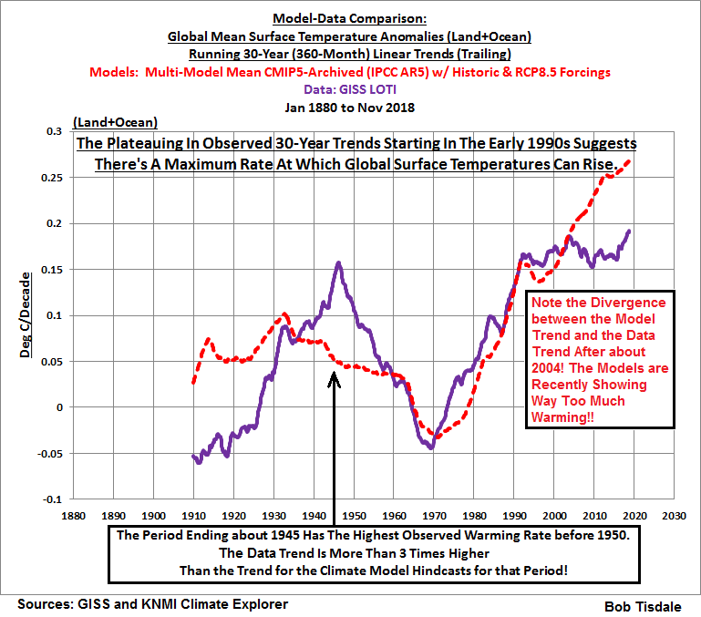
Figure 1

Figure 1 gives you an initial idea of how poorly the climate models simulate global surface temperatures during the early 20^th Century warming period of 1916-1945.  Note that the GISS Land-Ocean Temperature Index (LOTI) data indicate global surfaces [warned as] warmed at a rate of about +0.15 Deg C/decade for the period of 1916 to 1945, while the model outputs indicate they should have warmed at a much lower rate of about +0.05 deg C/decade if global temperatures were dictated by the forcings that are used to drive the number-crunching models.  Apparently multidecadal changes in global surface temperatures in the real world are not dictated by the forcings that drive the fantasy world models. Because the models, which are forced primarily by numerical representations of anthropogenic greenhouse gases, can’t explain the warming during that period, then the additional two-thirds of the warming that actually occurred during that period must have occurred naturally.  That of course raises the question: If two-thirds of the warming during period of 1916-1945 occurred naturally, is Mother Nature responsible for two-thirds of the observed warming during the latter part of the 20^th Century and into the early 21^st Century?  The fact that the models better align during the latter warming periods is immaterial, because climate models are tuned to that period, so the models cannot be verified or validated then.  The models can only be verified or validated—or invalidated, if you prefer—during periods outside of those they are tuned to, like the early warming period of 1916 to 1945.

A note for newcomers: The graph in Figure 1 is not how global mean surface temperature data are normally presented, so a graph like this may be confusing if you’re not familiar with it. For those requiring an explanation, first note the Title Block where the third line reads “Running 30-Year (360-Month) Linear Trends (Trailing)”.  Also note the units of the y-axis (the vertical axis) shown to the left of the graph.  The units are Deg C/Decade, not simply Deg C.   In other words, we’re illustrating trends in the graph: how quickly or how slowly global surfaces warmed or cooled over those 30-year periods.  The surface temperatures were rising if the data points are positive or falling if the data points are negative.   The greater a positive [negative] data point is, the faster the surface temperatures were rising [falling] over the 30-year period. Conversely, the closer a data point is to zero, the slower the surface temperatures were rising (positive data points) or falling (negative data points) over the 30-year period.  Also note the word “Trailing” in the third line of the title block.  That means the trend for every 30-year (actually 360-month) period is shown in its final month.  The x-axis, of course, is time in years.

If a series of data points is growing farther and farther away from zero with time, that means the 30-year trends are accelerating. Conversely, if a series of data points is growing closer and closer toward zero with time, that means the 30-year trends are decelerating.  That is, if the values are still positive, a drop with time in 30-year trends does not mean the surface temperatures are cooling. It shows that they are still warming but at a slower rate. To be showing cooling, the data points have to drop into negative values.

[End note.]

Figure 2 presents the 30-year trends in the GISS Land-Ocean Temperature Index (LOTI) data, using annual data. The fact that the 30-year period with the end year of 1945 has the highest 30-year warming rate before 1950 is clearer in Figure 2 than Figure 1.

Figure 2

In light of that, for the remainder of this post, I’m presenting data and the outputs of climate model simulations of the global mean surface temperatures (land+ocean, ocean only, and land-only) for the 30-year period of 1916 to 1945.

And for the remaining graphs in this post, I’m presenting normal time-series graphs, in which the units are degrees Celsius.

Later, after isolating four climate model ensemble members, I’ll present model-data comparisons of (1) global land near-surface air temperatures and (2) global sea surface temperatures.   Then, to end the post, I compare modeled marine air temperatures and sea surface temperatures for each of the 4 ensemble members.

A CLOSER LOOK AT OBSERVATIONS-BASED DATA

Figure 3 presents the annual global mean land+ocean surface temperature anomalies with data from Berkeley Earth—data here—and from NASA Goddard Institute for Space Studies (GISS)—data here. To better align the two datasets during this period, I’ve referenced the anomalies to the period of 1916-1945, so you can see the subtle differences between the two datasets.

Figure 3

The Berkeley Earth data have a slightly higher trend (+0.166 deg C/decade) than the GISS data (+0.153 deg C/decade).

CLIMATE MODEL OUTPUTS

As stated in the Introduction, the climate model outputs being presented are those stored in the Coupled Model Intercomparison Project Phase 5 (CMIP5) archives, which were used by the United Nations’ entity called the Intergovernmental Panel on Climate Change (IPCC) for their 5^th Assessment Report (AR5).  The models being presented are those with historic forcings through 2005 and RCP8.5 (worst-case scenario) forcings thereafter. The model outputs are available to the public through the KNMI Climate Explorer, specifically through the Monthly CMIP5 scenario runs webpage. (Thank you, Geert Jan van Oldenborgh, for that wonderful tool.)

Initially in this post, I’m presenting the climate model simulations of near surface air temperatures (identified as TAS at the KNMI Climate Explorer) for the latitudes of 90S-90N, and the longitudes of 180W-180E, in other words, globally.

Then after isolating the model ensemble members with the coolest and warmest outputs and the highest and lowest trends, we’ll compare observed and climate model simulations of global sea surface temperatures during the early warming period. At the KNMI Climate Explorer, the climate model simulations of sea surface temperatures are identified as “TOS”, assumedly for Temperature Ocean Surface.  Then we’ll use the simulations of near surface air temperatures again but isolate the land masses with the land/sea masking feature at the KNMI Climate Explorer.

You’ll note that I’ve identified the RCP forcings the modelers used after 2005 (RCP8.5) even though we’re looking at the climate model outputs for the 30-year period of 1916 to 1945. I’ve done this for persons who want to verify my results. The reason: The CMIP5 archive and the KNMI Climate Explorer contain the outputs of climate model simulations (runs) from the same models with the historic forcings through 2005 but with different RCP forcings after 2005.  The simulations of global mean surface temperatures may be different with each model run; in fact, they’re likely different.  So I wanted to make sure that anyone verifying the results was looking at the same model outputs.

BUT THE DATA EXCLUDE ANTARCTICA DURING THIS PERIOD WHILE THE MODELS INCLUDE ANTARCTICA

Anyone with a good understanding of the instrument temperature record will realize that little to no observations-based data exist for Antarctica before the early 1950s, so the Berkeley Earth and GISS datasets shown in Figures 1, 2, and 3 exclude observations from Antarctica. On the other hand, the climate model outputs presented in Figures 5 through 8 of this post are for the global land-ocean surfaces (90S-90N) so they do include Antarctica.

If that concerns you, see Figure 4. It presents the trends and period-averaged temperatures for the multi-model mean of the simulations of global land+ocean surface air temperatures from the models stored in the CMIP5 archive, for the period of 1916-1945, including and excluding Antarctica and the Southern Ocean. Also presented are the trend and period-averaged temperature for Antarctica and the Southern Ocean.

Figure 4

With or without Antarctica and the Southern Ocean, the trends of model-mean are basically the same. The difference is only one one-thousandths of a degree Celsius per decade (0.001 deg C/decade). The period-averaged temperatures are different, as one would expect with the cold continent of Antarctica. That is, without Antarctica and the Southern Ocean, modeled global mean near-surface air temperatures are a little more than 2 deg C higher than if they are included.

That explains why I did not present the data in Figure 3 above in observed (not anomaly) form…what the climate science industry would call absolute temperatures. Factors are available online to convert the Berkeley Earth and GISS global mean surface temperature data from anomalies back to the observed (not anomalies) form, but those factors are for the base period of 1951-1980, a period during which data from Antarctica are included.  I didn’t want to bother with an additional anomaly-to-not-anomaly factor for the data during 1916-1945 when Antarctic data are excluded.

The models, as you shall see, don’t need any additional help from me to look horrible.

Enough with the backstory…

THE INITIAL PRESENTATIONS OF THE CLIMATE MODEL OUTPUTS

Figure 5 presents the multi-model mean of the simulations of annual global mean land+ocean near-surface air temperatures. We present the multi-model mean because it represents the consensus (better said, the groupthink) of the climate modeling groups for how global near-surface air temperatures should have warmed IF (big if) they were dictated by the forcings that drive the models.  The curve in Figure 5 is the same curve as the light-blue one in Figure 4, but it looks much more dramatic in Figure 5 because of the tighter range of temperatures in the y-axis.

Figure 5

As discussed and illustrated earlier, the Berkeley Earth and the GISS observations-based data indicate global mean surface temperatures warmed at a rate that was more than 3 times faster than hindcast by the models for the period of 1916-1945. That’s a pretty horrendous display of modeling capabilities. In plain words, the disparity between the observed and modeled global mean surface warming rates during this early 20^th Century warming period indicates that the climate-science industry has no idea whatsoever about what causes global surfaces to change over multidecadal periods, none whatsoever.

As noted in red in Figure 5, a multi-model mean can be misleading, inasmuch as it gives the false impression of an agreement among models in terms of temperatures and trends. See Figure 6.  The multi-colored spaghetti graph in Figure 6 presents the curves of all 81 ensemble members that make up the multi-model mean in Figure 5.

Figure 6

As is obvious, the span of the period-averaged global mean surface temperatures of the climate models stored in the CMIP5 archive, with historic and RCP8.5 forcings, is greater than 3 deg C. The models surely have the actual surface temperatures surrounded, whatever they actually are during this period.  That 3-deg C span indicates the modelers have no idea what the global mean surface temperature is supposed to be during this period.

Figure 7 displays ensemble members with the warmest, coolest, and 2^nd coolest simulated global mean surface temperatures. They are the ensemble members identified at the KNMI Climate Explorer as GISS-E2-H p3, FGOALS-g2, and IPSL-CM5A-LR EM-1. Specifically:

• GISS-E2-H p3 is Warmest with a period-averaged global mean surface temperature of 15.4 deg C,
• FGOALS-g2 is Coolest with a period-averaged global mean surface temperature of 12.2 deg C, and,
• IPSL-CM5A-LR EM-1 is 2nd Coolest with a period-averaged global mean surface temperature of 12.4 deg C.

The difference in the period-averaged global mean surface temperatures, between the GISS-E2-H p3 (warmest) and FGOALS-g2 (coolest) ensemble members, is 3.2 deg C.

Figure 7

Note: The top 6 warmest models during this period are all products on the Goddard Institute for Space Studies (GISS). [End note.]

Now consider this: the 3+ deg C difference between the coolest and warmest models is about three times higher than the 1-deg C global warming that is said to have taken place since the end of the newly defined (by the IPCC) “pre-industrial” times.

The reason for presenting the 2^nd coolest ensemble member:  Later I break the models simulations of global mean surface temperatures down into their ocean and land components.  And, as we know, the ocean portion of the observations-based global mean surface temperature record relies on sea surface temperature data, not marine air temperature data.  Unfortunately, the KNMI Climate Explorer does not include the ocean surface temperature (TOS) output of the FGOALS-g2 ensemble member with historic and RCP8.5 forcings.  It does include, however, the ocean surface temperature output of the 2^nd coolest model IPSL-CM5A-LR EM-1, which will be our reference cool model in the following sections.

Note: The 6 GISS ensemble members with historic and RCP8.5 forcings are ranked 1^st to 6^th warmest, out of the 81 ensemble members with that mix of forcings. Now consider in climate models that (1) higher surface temperatures produce more evaporation and, in turn, more water vapor in the atmosphere, and (2) water vapor is a greenhouse gas.  Does the GISS Model E2 need warmer than actual surface temperatures in order to produce the politically motivated high future warming?

[End note.]

In the spaghetti graph in Figure 6 above, it was impossible to see the wide range of trends for the climate-model-simulated global mean surface temperatures during the period of 1916 to 1945.   Figure 8 includes the ensemble members with the highest and lowest trends in simulated global mean land-ocean near-surface air temperatures for the period of 1916-1945, based on the 81 ensemble members in the CMIP5 archive with historic and RCP8.5 forcings.  They are identified at the KNMI Climate Explorer as IPSL-CM5A-LR EM-2, and CMCC-CMS.  As relating to trends:

• IPSL-CM5A-LR EM-2 is the ensemble member with the highest trend, a warming rate of +0.151 deg C/decade, which is in line with the observations, and,
• CMCC-CMS is the ensemble member with the lowest trend, a cooling (yes, cooling) rate of -0.055 deg C/decade, which obviously is the wrong sign.

Figure 8

The IPSL-CM5A-LR EM-2, and CMCC-CMS will be the other two reference ensemble members for the land and ocean breakouts that follow.

Note: To expand on the discussion of trends, the multi-model mean (the consensus—a.k.a. groupthink—of the modeling groups) showed a trend of 0.05 deg C/decade for this early warming period, but the trends of the individual ensemble members ranged from +0.151 deg C/decade to -0.055 deg C per decade. Additionally, 6 other ensemble members had negative trends.  That is, the outputs of those six model runs indicated that global cooling should have been occurring during this period, if Earth’s surface temperatures were dictated by the forcings that drive the models. These are more examples of the horrendous modeling skills from the climate-science industry!  [End note.]

OBSERVED AND MODELED OCEAN SURFACE TEMPERATURES DURING THIS EARLY WARMING PERIOD

For references during this sea surface temperature breakout, we’re using HADISST1 data from the UK Met Office (UKMO) Hadley Centre and NOAA/NCEI’s updated “pause-buster 2” ERSST.v5 data, both of which are available at the KNMI Climate Explorer. The UKMO HADISST1 and NOAA “pause-buster 2” ERSST.v5 datasets are the sea surface temperature reconstructions that extend back past the period of 1916 to 1945 and that are presented in observed form, what the climate science industry calls “absolute” temperatures.

We’re limiting the latitudes to 60S-60N to eliminate the polar oceans with their sea ice. This is done because the data suppliers and modeling groups may account for sea ice differently. We also know that climate models do a terrible job of simulating sea ice area during the satellite era (See Figure Intro-8 and Figure Intro-9 on page 22 of my free ebook On Global Warming and the Illusions of Control-Part 1 here, 25MB in .pdf format.), so it’s best not to include the polar oceans in this discussion of sea surface temperatures. The Arctic Ocean (at 15,558,000 km²) and Southern Ocean (at 21,960,000 km²) represent roughly 10% of the surfaces of the global oceans (at 361,900,000 km²).  (The source or the ocean-surface-area data is the NOAA webpage here.) So, using the latitudes of 60S-60N, we’re including roughly 90% of the surfaces of the global oceans.

Figure 9 presents the observed global (60S-60N) sea surface temperatures and warming rates based on our two reference datasets, during the early 20^th Century warming period of 1916-1945.  The period-average temperatures are similar, at roughly 20 deg C.  The warming rates during this period are also similar, roughly +0.145 deg C/decade, with NOAA’s “pause-buster 2” sea surface temperature data having the higher warming rate at +0.155 deg C/decade…and the UKMO HADISST1 data having the lower trend at +0.135 deg C/decade.

Figure 9

The multi-model mean of the simulations of global (60S-60N) sea surface temperatures of the models stored in the CMIP5 archive with historic and RCP8.5 forcings is presented in Figure 10.

Figure 10

Knowing how poorly those same models simulate observed sea surface temperatures during the satellite era, I was surprised to see the modeled period-average global (60S-60N) sea surface temperatures as presented by the multi-model mean was similar to the observations. Then again, the simulated warming rate from the models is much too low at +0.038 deg C/decade.  Observations show the surfaces of the global oceans, excluding the polar oceans, warmed at a rate that was approximately 3.5 to 4 times higher than modeled.

Figure 11 presents the outputs of the GISS-E2-H p3, and IPSL-CM5A-LR EM-1 simulations of global (60S-60N) sea surface temperatures with the models using the historic and RCP8.5 forcings, for the period of 1916 to 1945. The difference in period average temperatures for the GISS-E2-H p3 and IPSL-CM5A-LR EM-1 ensemble members is about 2.8 deg C.

Figure 11

Then again, and as expected, the difference in the trends of simulated global (60S-60N) sea surface temperatures is eye opening. See Figure 12.  The IPSL-CM5A-LR EM-2 ensemble member shows that the global ocean surfaces should have warmed at a rate of +0.105 deg C/decade during the 30-year period of 1916-1945, which is noticeably less than observed, and the CMCC-CMS shows they should have cooled at a rate of -0.037 deg C/decade.

Figure 12

Considering that data indicate the surfaces of the ocean warmed at a rate of about +0.145 deg C/decade, those are pathetic modeling efforts.

OBSERVED AND MODELED LAND NEAR-SURFACE AIR TEMPERATURES AND TRENDS DURING THIS EARLY WARMING PERIOD

As noted earlier, observations based datasets do not include observations from Antarctica during this period. Regardless, I used the KNMI Climate Explorer to determine the observed global mean land near-surface air temperature anomalies for the latitudes of 60S-90N, eliminating Antarctica and any question of its influence on this presentation. And, because the GISS Land-Ocean Temperature Index (LOTI) dataset includes sea surface temperature data, I used the ocean masking feature of the KNMI Climate Explorer to extract only the land near-surface air temperature anomaly data for Figure 13, which compares that data to the Berkeley Earth (land only) surface temperature anomaly data.

Figure 13

I’ve used the period of 1916-1945 as reference for anomalies to better align the two datasets, so you can better see the differences. The Berkeley Earth data have a noticeably warmer trend at a rate of +0.177 deg C/decade, while the GISS data with oceans masked show a trend of +0.146 deg C/decade.

Then again, as shown in Figure 14, according to the model mean of the models stored in the CMIP5 archive with historic and RCP8.5 forcings, the global mean land near-surface air temperatures, excluding Antarctica, should only have warmed at a rate of +0.067 deg C/decade during this period. In other words, in the real world, from 1916 to 1945, global mean near-surface air temperatures for land masses warmed at a rate that was 2 to 2.5 times faster than the fantasy worlds of the average climate model ensemble member with this mix of forcings.

Figure 14

Note: I used the ocean-masking feature of the KNMI Climate Explorer to acquire the land-only portion of the climate model outputs. [End note.]

As shown in Figure 15, according to the IPSL-CM5A-LR EM-2 ensemble member, land near-surface air temperatures should have warmed at a rate of +0.212 deg C/decade, which is higher than observed, while the CMCC-CMS ensemble member shows a cooling trend of -0.054 deg C/decade. Remarkable!

Figure 15

Last but not least, as illustrated in Figure 16, we have the GISS-E2-H p3 with a period-average near-surface air temperature of 13.6 deg C and the IPSL-CM5A-LR EM-1 showing 11.1 deg C, for a span of 2.5 deg C. Well, with luck, they’ve got the actual near-surface air temperatures for the land masses surrounded, whatever they are.

Figure 16

IMPORTANT NOTE

Some readers may have recalled a temperature difference of 3.0 deg C between the GISS-E2-H p3 and IPSL-CM5A-LR EM-1 ensemble members when looking at global land+ocean near-surface air temperatures during this period as shown in Figure 7, while the temperature difference between those models for the ocean sea surface temperatures was 2.8 deg C (Figure 11) and, for land near-surface air temperatures, the difference was 2.5 deg C (Figure 16). Hmm. Something might not seem right to you.  Don’t worry.  Figure 11 presents modeled sea surface temperatures, while Figure 7 includes near-surface air temperatures for the oceans and land masses and Figure 17 shows near-surface air temperatures for land masses. And, sea surface temperatures and near-surface air temperatures are not the same…or consistently different in the models.

To set your mind at ease, Figure 17 presents the global (60S-60N) near-surface air temperatures for the oceans, what I’ve called Marine Air Temperature, which is not to be confused with the observations-based dataset Nighttime Marine Air Temperature or NMAT, which only includes observations at night. The difference in simulated Marine Air Temperatures between the GISS-E2-H p3 and IPSL-CM5A-LR EM-1 ensemble members is 3.2 deg C, which is more in line with what’s expected.

Figure 17

[End note.]

AND NOW FOR SOMETHING COMPLETELY…AMAZING

[Sorry, members of Monty Python, “And now for something completely different” just didn’t work.]

In Figures 18 to 22, I present the modeled global (60S-60N) sea surface temperatures and marine air temperatures (near-surface air temperatures with the land-surfaces masked). The curves for sea surface temperatures are solid and the marine air temperatures are dotted.  In all cases, the marine air temperatures are cooler than the sea surface temperatures.  The temperatures and temperature differences between the two, however, are not consistent, as you shall see.

Figure 18 includes the simulated global (60S-60N) mean sea surface temperature and marine air temperature of the multi-model mean of the climate models stored in the CMIP5 archive with historic and RCP8.5 forcings. According to the model-mean, which represents the group-think of the modeling groups, the marine air temperatures for the global oceans, excluding the polar oceans, should be 1.3 deg C cooler than the sea surface temperatures during the period of 1916-1945.

Figure 18

The two ensemble members from IPSL included in this post—IPSL-CM5A-LR EM-1 and IPSL-CM5A-LR EM-2—show a temperature difference of 1.6 deg C. See Figures 19 and 20.

Figure 19

# # #

Figure 20

Figure 21 includes the model-simulated temperatures for the two ocean metrics from the GISS-E2-H p3. Apparently, the GISS modelers believe the temperature difference between Marine Air Temperatures and Sea Surface Temperatures should be 1.1 deg C, not 1.6 deg C like the modelers who prepared the IPSL ensemble members.

Figure 21

But the modelers who prepared the CMCC-CMS ensemble member, as shown in Figure 22, believe the temperature difference between Marine Air Temperatures and Sea Surface Temperatures should be 0.8 deg C.

Figure 22

There you have it. More inconsistencies from the climate modeling groups.

AND NOAA SAYS

The following quote is from the NOAA Climate Models primer webpage.  It is the opening two sentences under the heading of “Climate Models and How They Work” (my boldface):

Climate models are based on well-documented physical processes to simulate the transfer of energy and materials through the climate system. Climate models, also known as general circulation models or GCMs, use mathematical equations to characterize how energy and matter interact in different parts of the ocean, atmosphere, land.…

Really? NOAA had the audacity to write that nonsense that “Climate models are based on well-documented physical processes…”, and yet, as we’ve just seen, the climate modeling groups can’t agree on a simple temperature difference between two interacting and coupled variables that physically touch one another, which are the surfaces of the global oceans and the near-surface air immediately above them.

BOTTOM LINE

Judith Curry wrote as the opening paragraph of her post Early 20th century global warming:

A careful look at the early 20th century global warming, which is almost as large as the warming since 1950.  Until we can explain the early 20th century warming, I have little confidence IPCC and NCA4 attribution statements regarding the cause of the recent warming.

Thank you, Judith. I won’t be as PC.

For the early 20^th Century 30-year warming period of 1916-1945, climate models are consistently horrible and consistently inconsistent at simulating the primary metric of human-induced climate change, which is global mean surface temperature.

And, surprisingly, based on those horrendous excuses for climate models, we’re supposed to believe their crystal-ball like prognostications of future global mean surface temperatures and other climate metrics!!?? Fat chance of that happening with anyone who has a spark of common sense.  If only more persons understood how poorly climate models simulated global mean surface temperatures—the primary metric of human-induced climate change—the human-induced global warming scare might just disappear into the past like the Y2K scare.  Then again, the global warming/climate change scare has nothing to do with science; it is simply global politics at its worst, masquerading as science.

That’s it for this post. Enjoy yourself in the comments and have a wonderful remainder of your day.

STANDARD CLOSING REQUEST

Please purchase my recently published ebooks. As many of you know, last year I published 2 ebooks that are available through Amazon in Kindle format:

• Dad, Why Are You A Global Warming Denier? (For an overview, the blog post that introduced it is here.)
• Dad, Is Climate Getting Worse in the United States? (See the blog post here for an overview.) In fact, one of the graphs at the beginning of this post (Exhibit 40) was from this ebook.WUWT LINKS
• And please purchase Anthony Watts’s et al. Climate Change: The Facts – 2017.

To those of you who have purchased them, thank you. To those of you who will purchase them, thank you, too.

Regards,

Bob Tisdale