On Cowtan and Way (2013) “Coverage bias in the HadCRUT4 temperature series and its impact on recent temperature trends”

INTRODUCTION

The recent paper by Cowtan and Way (2013) Coverage bias in the HadCRUT4 temperature series and its impact on recent temperature trends made the rounds in the climate change blogosphere. Posts at RealClimate (here) and at SkepticalScience (here) looked on the paper as the second coming of…errr…Hansen’s GISTEMP maybe, saying Cowtan and Way (2013) proved the UKMO HADCRUT4 data underreports by half the warming of global surface temperatures since 1997.  The posts at WattsUpWithThat (here) and at Judith Curry’s blog (here) weren’t so flattering, to put it mildly. Lucia at her blog TheBlackboard had three posts (here, here and here.)  Lucia spoke favorably about Cowtan and Way (2013), but offered in a comment (here):

That said: We do need to put the changes in context of testing models, and they don’t make a big difference. Models still look pretty bad, though maybe a tiny bit less bad. If the models are bad we can be pretty confident the divergence will increase over time — though it might take longer. OTOH: if the models are ok, the divergence will correct itself. Observing this puts us exactly where we were before C&W was published!

And Steve McIntyre’s post (here) illustrated the apparent 2005 breakpoint in his Figure 2.  I’ll discuss in this post why that’s odd, among other things.

Unlike GISS and NCDC global surface temperature datasets, HADCRUT4 data are not infilled. That is, if there are no temperature measurements in a 5 deg latitude by 5 deg longitude grid for a given month, that grid is left blank in the HADCRUT4 dataset.  GISS and NCDC infill most of the missing grids using different statistical tools (with NCDC exclusing the polar sea ice).

Cowtan and Way (2013) used two methods to infill the missing grids in the HADCRUT4 dataset.  One is called Kriging. (See the Wikipedia page here.)  With the other, they used Lower Troposphere Temperature data from UAH (the Spencer and Christy data) as a source to fill in the blanks. This latter version is called the hybrid version by Cowtan and Way (2013). Their focus appears to be the Arctic, where polar amplification has land surface temperatures warming at an accelerated rate.

Cowtan and Way explain in their post at SkepticalScience:

In their paper, Cowtan & Way apply a kriging approach to fill in the gaps between surface measurements, but they do so for both land and oceans. In a second approach, they also take advantage of the near-global coverage of satellite observations, combining the University of Alabama at Huntsville (UAH) satellite temperature measurements with the available surface data to fill in the gaps with a ‘hybrid’ temperature data set. They found that the kriging method works best to estimate temperatures over the oceans, while the hybrid method works best over land and most importantly sea ice, which accounts for much of the unobserved region.

The basic assumption behind the Cowtan and Way (2013) paper appears to be, because the HADCRUT4 data doesn’t capture the Arctic Ocean (there are no temperature measurements there other than sea surface temperatures when sea ice melts seasonally), the warming in the Arctic is underreported.  As a result, the global warming since 1997 in the HADCRUT4 data is too low, because they fail to show the additional warming in the Arctic.

Both methods used by Cowtan and Way (2013) produced curious results, as we shall discuss.

A COUPLE OF QUICK COMPARISONS

As an introduction, Figures 1 and 2 compare the HADCRUT4 data (combined global land air plus sea surface temperature anomalies) to the two datasets from Cowtan and Way (2013). The base years for anomalies are 1981-2010. The source of the Cowtan and Way (2013) data is here, and I used the KNMI Climate Explorer for the HADCRUT4 data.   The comparisons for the full 1979 to 2012 term of the Cowtan and Way (2013) are in the left-hand graphs and the “hiatus period” of 1997 to 2012 are shown in the right-hand graphs.  (Click on the graphs for larger illustrations.)

Figure 1

# # #

Figure 2

Both versions of the Cowtan and Way (2013) data have slightly higher long-term (1979-2012) warming rates than HADCRUT4, but they have much higher warming rates than HADCRUT4 during the hiatus period of 1997-2012.  Of course, this the reason it is praised by global warming enthisiasts.

DIFFERENCES BETWEEN HADCRUT4 AND COWTAN AND WAY DATA PRESENT CURIOUS RESULTS

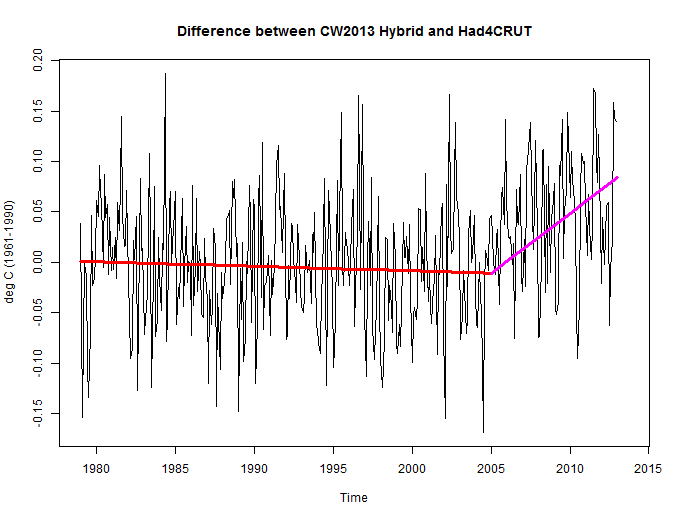
Figure 3 presents two graphs showing the differences between the HADCRUT4 data and the two versions of the Cowtan and Way (2013) data.  Note the apparent breakpoint around 2005 with both datasets.

Figure 3

I’ve divided the difference graphs into two periods, January 1979 to December 2004, and January 2005 to December 2012. See Figure 4.

Figure 4

Steve McIntyre noticed the same breakpoint.  See Steve’s Figure 2 here.

As you’ll note, the differences shows negative trends before 2005.  That means the HADCRUT4 data are warming faster than the Cowtan and Way (2013) data. Then after 2005, the differences are showing positive trends, meaning the Cowtan and Way (2013) data are warming faster than the HADCRUT4 data.

The results are odd.

Why?  The Cowtan and Way (2013) datasets were intended to produce polar amplification.  Cowtan and Way, in their blog post at SkepticalScience, write:

Both of their new surface temperature data sets show significantly more warming over the past 16 years than HadCRUT4. This is mainly due to HadCRUT4 missing accelerated Arctic warming, especially since 1997.

Stefan Rahmstorf, in his post at RealClimate, explains in the opening 4 paragraphs of that post (His boldface):

A new study by British and Canadian researchers shows that the global temperature rise of the past 15 years has been greatly underestimated. The reason is the data gaps in the weather station network, especially in the Arctic. If you fill these data gaps using satellite measurements, the warming trend is more than doubled in the widely used HadCRUT4 data, and the much-discussed “warming pause” has virtually disappeared.

Obtaining the globally averaged temperature from weather station data has a well-known problem: there are some gaps in the data, especially in the polar regions and in parts of Africa. As long as the regions not covered warm up like the rest of the world, that does not change the global temperature curve.

But errors in global temperature trends arise if these areas evolve differently from the global mean. That’s been the case over the last 15 years in the Arctic, which has warmed exceptionally fast, as shown by satellite and reanalysis data and by the massive sea ice loss there. This problem was analysed for the first time by Rasmus in 2008 at RealClimate, and it was later confirmed by other authors in the scientific literature.

The “Arctic hole” is the main reason for the difference between the NASA GISS data and the other two data sets of near-surface temperature, HadCRUT and NOAA. I have always preferred the GISS data because NASA fills the data gaps by interpolation from the edges, which is certainly better than not filling them at all.

But according to the differences between the HADCRUT4 and Cowtan and Way (2013) datasets, Figure 4, the HADCRUT4 data warms faster than the Cowtan and Way (2013) datasets before 2005. That is, we’re not seeing the impacts of the polar amplification before 2005

We can look at the impacts of the GISS infilling method by subtracting the global GISS land-ocean temperature index data with 250km smoothing from the GISS data with 1200km smoothing. See Figure 5.  I’ve also broken the difference results into the same two periods as Figure 4, before and after 2005.

Figure 5

The GISS relationship is what we would expect.  Northern Hemisphere surface temperatures have been warming since the mid-1970s. Polar amplification exaggerated that warming in the Arctic. So the infilled GISS data, which extends out over the Arctic, would show the greater warming since the 1970s…until the warming stops for Northern Hemisphere sea surface temperatures and for the low-to-mid latitude land surface air temperatures.  See Figure 6.

Figure 6

The left-hand graph in Figure 6 presents the GISS Land-Ocean Temperature Index (LOTI) data for the low-to-mid latitudes of the Northern Hemisphere (0-65N). The ocean data was masked (one of the features of the KNMI Climate Explorer with the GISS LOTI data).  Land surface air temperatures there effectively stopped warming around 1998. The right-hand graph in Figure 6 presents the Northern Hemisphere GISS sea surface temperature anomalies.  For it, the land surface temperature data was masked. GISS also masks sea surface temperature wherever sea ice has existed so there is little data in the Arctic Ocean.  The GISS Northern Hemisphere sea surface temperature data appears to have peaked around 2005.  So the additional the warming of the infilled GISS data before 1995 and the slowing afterwards(Figure 5) appears to make sense.

That suggests that the infilling methods used by Cowtan and Way (2013), shown in Figure 4, provide results that aren’t realistic.   That of course assumes that the primary reason for the differences between the HADCRUT4 data and the Cowtan and Way (2013) data is the Arctic data—as Cowtan and Way and as Stefan Rahmstorf have portrayed.

THE COWTAN AND WAY DATA DO NOT HELP CLIMATE MODELS

The Cowtan and Way (2013) data are not available on a gridded basis in an easy-to-use format.  So we’ll be presenting the HADCRUT3 data along with a few other datasets as references in this section.  We’ll also be presenting the warming and cooling rates (the trends) on a zonal means (latitude average) basis.

For example, Figure 7 illustrates the warming and cooling rates of the HADCRUT4 data, and as a reference, the GISS LOTI data, for the period of January 1997 to December 2012…the hiatus period. The vertical axis (y-axis) is scaled in deg C/decade, so we’re showing the warming and cooling rates or trends. The horizontal axis (x-axis) is scaled in latitude, so the South Pole is to the left at -90 (90S) and North Pole is to the right at 90 (90N). Both datasets show the very slow warming rates (and cooling at some latitudes) extending from the mid-latitudes of the Southern Hemisphere to the mid-latitudes of the Northern Hemisphere.  Both poles show continued warming.

Figure 7

Background Information:  Climate models, on the other hand, have difficulty with polar amplification. They do not simulate it properly.  Figure 8 presents model-data trend comparisons for the two warming periods since 1914 and the warming hiatus period from 1945 to 1975. (The illustrations are from my book Climate Models Fail.)  The models do a reasonable job of portraying the polar amplification shown by the GISS LOTI data from 1975 to 2012, as illustrated in the upper left-hand graph.  But the models fail to capture the polar-amplified cooling in the Arctic from 1945 to 1975 (upper right-hand graph), and they definitely do not show the polar-amplified warming that occurred from 1914 to 1945 (lower left-hand graph).

Figure 8

If we compare the HADCRUT4 data to the CMIP5 models (historic and RCP6.0) for the period of 1997 to 2012, Figure 9, we can see that the models over-estimate the warming from 65S to 65N (the vast majority of the planet) and underestimate the warming at the poles.  Therefore, if the Cowtan and Way (2013) data are increasing the warming in the Arctic, they are creating a greater divergence from the models there, but failing to reduce the differences between the models and data where the models overestimate the warming.

Figure 9

Additional note: The following is a portion of Chapter from my book Climate Models Fail.  It seems appropriate for this discussion:

There is a remarkable paper that explains why the current generation of climate models (CMIP5) is in better agreement among themselves than the previous generation (CMIP3) but, as a result, they perform worse. See Swanson (2013) “Emerging Selection Bias in Large-scale Climate Change Simulations.” The preprint version of the paper is here. In the Introduction, Swanson writes (my boldface):

Here we suggest the possibility that a selection bias based upon warming rate is emerging in the enterprise of large-scale climate change simulation. Instead of involving a choice of whether to keep or discard an observation based upon a prior expectation, we hypothesize that this selection bias involves the ‘survival’ of climate models from generation to generation, based upon their warming rate. One plausible explanation suggests this bias originates in the desirable goal to more accurately capture the most spectacular observed manifestation of recent warming, namely the ongoing Arctic amplification of warming and accompanying collapse in Arctic sea ice. However, fidelity to the observed Arctic warming is not equivalent to fidelity in capturing the overall pattern of climate warming. As aresult, the current generation (CMIP5) model ensemble mean performsworse at capturing the observed latitudinal structure of warming than theearlier generation (CMIP3) model ensemble. This is despite a markedreduction in the inter-ensemble spread going from CMIP3 to CMIP5, whichby itself indicates higher confidence in the consensus solution. In otherwords, CMIP5 simulations viewed in aggregate appear to provide a moreprecise, but less accurate picture of actual climate warming compared toCMIP3.

In other words, the current generation of climate models (CMIP5) agrees better among themselves than the prior generation (CMIP3), i.e., there is less of a spread between climate model outputs, because they are converging on the same results. Overall, however, the CMIP5 models perform worse than the than the prior generation, CMIP3.

According to Swanson (2013) modelers made the models worse throughout most of the globe in efforts to create more warming in the Arctic. So by increasing the warming in the Arctic, Cowtan and Way have not helped the models.

USING LOWER TROPSPHERE TEMPERATURE DATA TO INFILL SURFACE TEMPERATURE DATA

The hybrid method used by Cowtan and Way (2013) fills in missing data (both land air and sea surface temperature) using lower troposphere temperature data from UAH.  Lower troposphere temperature data represents the temperature of the atmosphere at approximately 3000 meters above sea level, as determined by satellite measurements.   The lower troposphere temperature data are spatially complete by comparison to surface temperature measurements.

As noted earlier, in their post at SkepticalScience, Cowtan and Way write:

They found that the kriging method works best to estimate temperatures over the oceans, while the hybrid method works best over land and most importantly sea ice, which accounts for much of the unobserved region.

It’s hard to imagine how Cowtan and Way could determine with any degree of certainty how “the hybrid method works best over land and most importantly sea ice” when there is so little surface air temperature data over sea ice.  If Cowtan and Way are using reanalyses as references, reanalyses use climate models to infill the missing data, so reanalyses also are not observations-based data out over the Arctic and Southern Oceans.  Reanalyses are simply another way of infilling.

Animation 1 compares the GISS land surface air temperature trends to UAH lower troposphere temperature trends over land for the period of 1979 to 2012. The ocean data for both datasets have been masked.  We’re using GISS LOTI data because it’s more spatially complete than the UKMO CRUTEM data (which is used in the HADCRUT4 data). The spatial patterns of the warming of both datasets are similar in some places but quite different in others. Assuming the spatial patterns of the warming shown by the GISS LOTI data are close to being correct, then the differences with the lower troposphere data appear to show that lower troposphere temperature data would be of questionable value for infilling the HADCRUT4 data.

Animation 1

The differences in the warming spatial patterns are even more pronounced for the period of 1997 to 2012.  See Animation 2. It’s hard to imagine using lower troposphere temperature data to infill land surface air temperature data.

Animation 2

Let’s compare the warming and cooling patterns for lower troposphere temperatures over the oceans to a spatially complete, satellite-enhanced sea surface temperature dataset, Reynolds OI.v2. Because the Reynolds OI.v2 data starts in November 1981, the trend analysis in Animation 3 covers the period of 1982 to 2012. There are few similarities in the warming and cooling patterns.

Animation 3

And for the period of 1997 to 2012, there are no similarities between the warming and cooling patterns for lower troposphere temperatures over the oceans and the satellite-enhanced sea surface temperature data.

Animation 4

Based on the dissimilarities between the warming and cooling patterns of the lower troposphere temperature and surface temperature data, it appears using lower troposphere temperature data to infill surface temperature data would provide erroneous results.

I also suspect that a good portion of the additional warming shown in the hybrid version of the Cowtan and Way (2013) data (versus their Krig data) comes from the Southern Ocean surrounding Antarctica, where sea surface temperatures are cooling and lower troposphere temperatures are warming.

One last comparison graph, as a reference for discussion:  Figure 10 compares the trends from 1997 to 2012 of GISS LOTI, HADCRUT4 and UAH Lower Troposphere Temperature anomalies. Curiously, since 1997, the UAH lower troposphere temperature data shows less warming in the Arctic than the GISS and HADCRUT4 data.  And the lower troposphere temperatures also show warming in the Southern Ocean (latitudes 65S-55S) while the surface temperature-based datasets both show cooling.

Figure 10

A FINAL NOTE

I’ve used GISS LOTI data in this post as a reference. That does not mean I agree with the way GISS treats the Arctic and Southern Oceans.  GISS masks (effectively deletes) sea surface temperature data anywhere sea ice has existed.  They then infill the Arctic and Southern Oceans with land surface air temperature data. While this is logical in winter, when sea ice exists on the oceans and snow cover exists on land surfaces, it is not logical during the summer, when seasonal sea ice melt exposes the open ocean, and when snow melt exposes land surface.  Sea surface temperatures vary at a much lower rate than land surface temperatures. And air temperatures over exposed land surfaces should warm differently than air temperatures over sea ice, especially when open ocean separates them. GISS data in the Arctic and Southern Oceans, therefore, would exaggerate the warming in both polar oceans.

CLOSING

The datasets produced by Cowtan and Way (2013) do not appear to provide polar amplification for the period of 1979 to 2004, because the HADCRUT4 data warmed faster than the Cowtan and Way (2013) data before 2005.  See the discussions of Figures 3, 4 and 5.

Increasing polar-amplified warming in the Arctic does not help climate models, which show poor polar amplification results.  Refer to the discussions of Figures 7, 8 and 9.

And due to the differences in the spatial patterns of warming and cooling, using lower troposphere temperatures to infill surface temperature data appears questionable.

As I was writing this post, Judith Curry also published the post Uncertainty in Arctic temperatures.  It’s definitely worth reading in light of Cowtan and Way (2013).