
UPDATE 2: Animation 1 from this post is happily displaying the differences between the “Best” models and observations in the first comment at a well-known alarmist blog. Please see update 2 at the end of this post.
# # # #
UPDATE: Please see the update at the end of the post.
# # #
 The new paper Risbey et al. (2014) will likely be very controversial based solely on the two co-authors identified in the title above (and shown in the photos to the right). As a result, I suspect it will garner a lot of attention…a lot of attention. This post is not about those two controversial authors, though their contributions to the paper are discussed. This post is about the numerous curiosities in the paper. For those new to discussions of global warming, I’ve tried to make this post as non-technical as possible, but these are comments on a scientific paper.
OVERVIEW
The Risbey et al. (2014) Well-estimated global surface warming in climate projections selected for ENSO phase is yet another paper trying to blame the recent dominance of La Niña events for the slowdown in global surface temperature warming, the hiatus. This one, however, states that ENSO contributes to the warming when El Niño events dominate. That occurred from the mid-1970s to the late-1990s. Risbey et al. (2014) also has a number of curiosities that make it stand out from the rest. One of those curiosities is that they claim that 4 specially selected climate models (which they failed to identify) can reproduce the spatial patterns of warming and cooling in the Pacific (and the rest of the ocean basins) during the hiatus period, while the maps they presented of observed versus modeled trends contradict the claims.
IMPORTANT INITIAL NOTE
I’ve read and reread Risbey et al. (2014) a number of times and I can’t find where they identify the “best” 4 and “worst” 4 climate models presented in their Figure 5. I asked Anthony Watts to provide a second set of eyes, and he was also unable to find where they list the models selected for that illustration.
Risbey et al. (2014) identify 18 models, but not the “best” and “worst” of those 18 they used in their Figure 5. Please let me know if I’ve somehow overlooked them. I’ll then strike any related text in this post.
Further to this topic, Anthony Watts sent emails to two of the authors on Friday, July 18, 2014, asking if the models selected for Figure 5 had been named somewhere. Refer to Anthony’s post A courtesy note ahead of publication for Risbey et al. 2014. Anthony has not received replies. While there are numerous other 15-year periods presented in Risbey et al (2014) along with numerous other “best” and “worst” models, our questions pertained solely to Figure 5 and the period of 1998-2012, so it should have been relatively easy to answer the question…and one would have thought the models would have been identified in the Supplementary Information for the paper, but there is no Supplementary Information.
Because Risbey et al. (2014) have not identified the models they’ve selected as “best” and “worst”, their work cannot be verified.
INTRODUCTION
The Risbey et al. (2014) paper Well-estimated global surface warming in climate projections selected for ENSO phase was just published online. Risbey et al. (2014) are claiming that if they cherry-pick a few climate models from the CMIP5 archive (used by the IPCC for their 5th Assessment Report)—that is, if they select specific climate models that best simulate a dominance of La Niña events during the global warming hiatus period of 1998 to 2012—then those models provide a good estimate of warming trends (or lack thereof) and those models also properly simulate the sea surface temperature patterns in the Pacific, and elsewhere.
Those are very odd claims. The spatial patterns of warming and cooling in the Pacific are dictated primarily by ENSO processes and climate models still can’t simulate the most basic of ENSO processes. Even if a few of the models created the warning and cooling spatial patterns by some freak occurrence, the models still do not (cannot) properly simulate ENSO processes. In that respect, the findings of Risbey et al. (2014) are pointless.
Additionally, their claims that the very-small, cherry-picked subset of climate models provides good estimates of the spatial patterns of warming and cooling in the Pacific for the period of 1998-2012 are not supported by the data and model outputs they presented, so Risbey et al. (2014) failed to deliver.
There are a number of other curiosities, too.
ABSTRACT
The Risbey et al. (2014) abstract reads (my boldface):
The question of how climate model projections have tracked the actual evolution of global mean surface air temperature is important in establishing the credibility of their projections. Some studies and the IPCC Fifth Assessment Report suggest that the recent 15-year period (1998–2012) provides evidence that models are overestimating current temperature evolution. Such comparisons are not evidence against model trends because they represent only one realization where the decadal natural variability component of the model climate is generally not in phase with observations. We present a more appropriate test of models where only those models with natural variability (represented by El Niño/Southern Oscillation) largely in phase with observations are selected from multi-model ensembles for comparison with observations. These tests show that climate models have provided good estimates of 15-year trends, including for recent periods and for Pacific spatial trend patterns.
Curiously, in their abstract, Risbey et al. (2014) note a major flaw with the climate models used by the IPCC for their 5th Assessment Report—that they are “generally not in phase with observations”—but they don’t accept that as a flaw. If your stock broker’s models were out of phase with observations, would you continue to invest with that broker based on their out-of-phase models or would you look for another broker whose models were in-phase with observations? Of course, you’d look elsewhere.
Unfortunately, we don’t have any other climate “broker” models to choose from. There are no climate models that can simulate naturally occurring coupled ocean-atmosphere processes that can contribute to global warming and that can stop global warming…or, obviously, simulate those processes in-phase with the real world. Yet governments around the globe continue to invest billions annually in out-of-phase models.
Risbey et al. (2014), like numerous other papers, are basically attempting to blame a shift in ENSO dominance (from a dominance of El Niño events to a dominance of La Niña events) for the recent slowdown in the warming of surface temperatures. Unlike others, they acknowledge that ENSO would also have contributed to the warming from the mid-1970s to the late 1990s, a period when El Niños dominated.
CHANCE VERSUS SKILL
The fifth paragraph of Risbey et al. (2014) begins (my boldface):
In the CMIP5 models run using historical forcing there is no way to ensure that the model has the same sequence of ENSO events as the real world. This will occur only by chance and only for limited periods, because natural variability in the models is not constrained to occur in the same sequence as the real world.
Risbey et al. (2014) admitted that the models they selected for having the proper sequence of ENSO events did so by chance, not out of skill, which undermines the intent of their paper. If the focus of the paper had been need for climate models to be in-phase with obseervations, they would have achieved their goal. But that wasn’t the aim of the paper. The concluding sentence of the abstract claims that “…climate models have provided good estimates of 15-year trends, including for recent periods…” when, in fact, it was by pure chance that the cherry-picked models aligned with the real world. No skill involved. If models had any skill, the outputs of the models would be in-phase with observations.
ENSO CONTRIBUTES TO WARMING
The fifth paragraph of the paper continues:
For any 15-year period the rate of warming in the real world may accelerate or decelerate depending on the phase of ENSO predominant over the period.
Risbey et al. (2014) admitted with that sentence, if a dominance of La Niña events can cause surface warming to slow (“decelerate”), then a dominance of El Niño events can provide a naturally occurring and naturally fueled contribution to global warming (“accelerate” it), above and beyond the forced component of the models. Unfortunately, climate models were tuned to a period when El Niño events dominated (the mid-1970s to the late 1990s), yet climate modelers assumed all of the warming during that period was caused by manmade greenhouse gases. (See the discussion of Figure 9.5 from the IPCC’s 4th Assessment Report here and Chapter 9 from AR4 here.) As a result, the models have grossly overestimated the forced component of the warming and, in turn, climate sensitivity.
Some might believe that Risbey et al (2014) have thrown the IPCC under the bus, so to speak. But I don’t believe so. We’ll have to see how the mainstream media responds to the paper. I don’t think the media will even catch the significance of ENSO contributions to warming since science reporters have not been very forthcoming about the failings of climate science.
Risbey et al (2014) have also overlooked the contribution of the Atlantic Multidecadal Oscillation during the period to which climate models were tuned. From the mid-1970s to the early-2000s, the additional naturally occurring warming of the sea surface temperatures of the North Atlantic contributed considerably to the warming of sea surface temperatures of the Northern Hemisphere (and in turn to land surface air temperatures). This also adds to the overestimation of the forced component of the warming (and climate sensitivity) during the recent warming period. Sea surface temperatures in the North Atlantic have also been flat for the past decade, suggesting that the Atlantic Multidecadal Oscillation has ended its contribution to global warming, and, because by definition the Atlantic Multidecadal Oscillation lasts for multiple decades, the sea surface temperatures of the North Atlantic may continue to remain flat or even cool for another couple of decades. (See the NOAA Frequently Asked Questions About the Atlantic Multidecadal Oscillation (AMO) webpage and the posts An Introduction To ENSO, AMO, and PDO — Part 2 and Multidecadal Variations and Sea Surface Temperature Reconstructions.)
For more than 5 years, I have gone to great lengths to illustrate and explain how El Niño and La Niña processes contributed to the warming of sea surface temperatures and the oceans to depth. If this topic is new to you, see my free illustrated essay “The Manmade Global Warming Challenge” (42mb). Recently Kevin Trenberth acknowledged that strong El Niño events cause upward steps in global surface temperatures. Refer to the post The 2014/15 El Niño – Part 9 – Kevin Trenberth is Looking Forward to Another “Big Jump”. And now the authors of Risbey et al. (2014)—including the two activists Stephan Lewandowsky and Naomi Oreskes—are admitting that ENSO can contribute to global warming. How many more years will pass before mainstream media and politicians acknowledge that nature can and does provide a major contribution to global warming? Or should that be how many more decades will pass?
RISBEY ET AL. (2014) – AN EXERCISE IN FUTILITY
IF (big if) the climate models in the CMIP5 archive were capable of simulating the coupled ocean-atmosphere processes associated with El Niño and La Niña events (collectively called ENSO processes hereafter), Risbey et al (2014) might have value…if the intent of their paper was to point out that models need to be in-phase with nature. Then, even though all of the models do not properly simulate the timing, strength or duration of ENSO events, Risbey et al (2014) could have selected, as they have done, specific models that best simulated ENSO during the hiatus period.
However, climate models cannot properly simulate ENSO processes, even the most basic of processes like Bjerknes feedback. (Bjerknes feedback, basically, is the positive feedback between the trade wind strength and sea surface temperature gradient from east to west in the equatorial Pacific.) These model failings have been known for years. See Guilyardi et al. (2009)and Bellenger et al (2012). It is very difficult to find a portion—any portion—of ENSO processes that climate models simulate properly. Therefore, the fact that Risbey et al (2014) selected models that better simulate the ENSO trends for the period of 1998 to 2012 is pointless, because the models are not correctly simulating ENSO processes. The models are creating variations in the sea surface temperatures of the tropical Pacific but that “noise” has no relationship to El Niño and La Nina processes as they exist in nature.
Oddly, Risbey et al (2014) acknowledge that the models do not properly simulate ENSO processes. The start of the last paragraph under the heading of “Phase-selected projections” reads [Reference 28 is Guilyardi et al. (2009)]:
This method of phase aligning to select appropriate model trend estimates will not be perfect as the models contain errors in the forcing histories27 and errors in the simulation of ENSO (refs 25, 28) and other processes.
The climate model failings with respect to how they simulate ENSO aren’t minor errors. They are catastrophic model failings, yet the IPCC hasn’t come to terms with the importance of those flaws yet. On the other hand, the authors of Guilyardi et al. (2009) were quite clear in their understandings of those climate model failings, when they wrote:
Because ENSO is the dominant mode of climate variability at interannual time scales, the lack of consistency in the model predictions of the response of ENSO to global warming currently limits our confidence in using these predictions to address adaptive societal concerns, such as regional impacts or extremes (Joseph and Nigam 2006; Power et al. 2006).
ENSO is one of the primary processes through which heat is distributed from the tropics to the poles. Those processes are chaotic and they vary over annual, decadal and multidecadal time periods.
During some multidecadal periods, El Niño events dominate. During others, La Niña events are dominant. During the multidecadal periods when El Niño events dominate:
- ENSO processes release more heat than “normal” from the tropical Pacific to the atmosphere, and
- ENSO processes redistribute more warm water than “normal” from the tropical Pacific to adjoining ocean basins, and
- through teleconnections, ENSO processes cause less evaporative cooling from, and more sunlight than “normal” to reach into, remote ocean basins, both of which result in ocean warming at the surface and to depth.
As a result, during multidecadal periods when El Niño events dominate, like the period from the mid-1970s to the late 1990s, global surface temperatures and ocean heat content rise. In other words, global warming occurs. There is no way global warming cannot occur during a period when El Niño events dominate. But projections of future global warming and climate change based on climate models don’t account for that naturally caused warming because the models cannot simulate ENSO processes…or teleconnections.
Now that ENSO has switched modes so that La Niña events are dominant the climate-science community is scrambling to explain the loss of naturally caused warming, which they’ve been blaming on manmade greenhouse gases all along.
RISBEY ET AL. (2014) FAIL TO DELIVER
Risbey et al (2014) selected 18 climate models from the 38 contained in the CMIP5 archive for the majority of their study. Under the heading of “Methods”, they listed all of the models in the CMIP5 archive and boldfaced the models they selected:
The set of CMIP5 models used are: ACCESS1-0, ACCESS1-3, bcc-csm1-1, bcc-csm1-1-m, BNU-ESM, CanESM2, CCSM4, CESM1-BGC, CESM1-CAM5, CMCC-CM, CMCC-CMS, CNRM-CM5, CSIRO-Mk3-6-0, EC-EARTH, FGOALS-s2, FIO-ESM, GFDL-CM3, GFDL-ESM2G, GFDL-ESM2M, GISS-E2-H, GISS-E2-H-CC, GISS-E2-R, GISS-E2-R-CC, HadGEM2-AO, HadGEM2-CC, HadGEM2-ES, INMCM4, IPSL-CM5A-LR, IPSL-CM5A-MR, IPSL-CM5B-LR, MIROC-ESM, MIROC-ESM-CHEM, MIROC5, MPI-ESM-LR, MPI-ESM-MR, MRI-CGCM3, NorESM1-M and NorESM1-ME.
Those 18 were selected because model outputs of sea surface temperatures for the NINO3.4 region were available from those models:
A subset of 18 of the 38 CMIP5 models were available to us with SST data to compute Niño3.4 (ref. 24) indices.
For their evaluation of warming and cooling trends, spatially, during the hiatus period of 1998 to 2012, Risbey et al (2014) whittled the number down to 4 models that “best” simulated the trends and 4 models that simulated the trends “worst”. They define how those “best” and “worst” models were selected:
To select this subset of models for any 15-year period, we calculate the 15-year trend in Niño3.4 index24 in observations and in CMIP5 models and select only those models with a Niño3.4 trend within a tolerance window of +/- 0.01K y-1 of the observed Niño3.4 trend. This approach ensures that we select only models with a phasing of ENSO regime and ocean heat uptake largely in line with observations. In this case we select the subset of models in phase with observations from a reduced set of 18 CMIP5 models where Niño3.4 data were available25 and for the period since 1950 when Niño3.4 indices are more reliable in observations.
The opening phrase of “To select this subset of models for any 15-year period…” indicates the “best” and “worst” models varied depending on the 15-year time period. Risbey et al. (2014) presented the period of 1998 to 2012 for their Figure 5. But in other discussions, like for those of their Figures 4 and 6, the number of “best” and “worst” models changed as did the models. The caption for their Figure 4 includes:
The blue dots (a,c) show the 15-year average trends from only those CMIP5 runs in each 15-year period where the model Niño3.4 trend is close to the observed Niño3.4 trend. The size of the blue dot is proportional to the number of models selected. If fewer than two models are selected in a period, they are not included in the plot. The blue envelope is a 2.5–97.5 percentile loess-smoothed fit to the model 15-year trends weighted by the number of models at each point. b and d contain the same observed trends in red for GISS and Cowtan and Way respectively. The grey dots show the average 15-year trends for only the models with the worst correspondence to the observed Niño3.4 trend. The grey envelope in b and d is defined as for the blue envelope in a and c. Results for HadCRUT4 (not shown) are broadly similar to those of Cowtan and Way.
That is, the “best” models and the number of them changes for each 15-year period. In other words, they’ve used a sort of running cherry-pick for the models in their Figure 4. A novel approach. Somehow, though, this gets highlighted in the abstract as “These tests show that climate models have provided good estimates of 15-year trends, including for recent periods and for Pacific spatial trend patterns.” But they failed to highlight the real findings of their paper: that climate models must be in-phase with nature if the models are to have value.
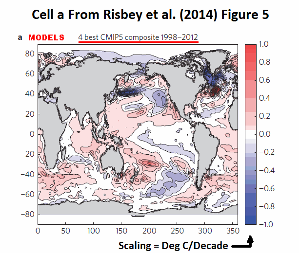
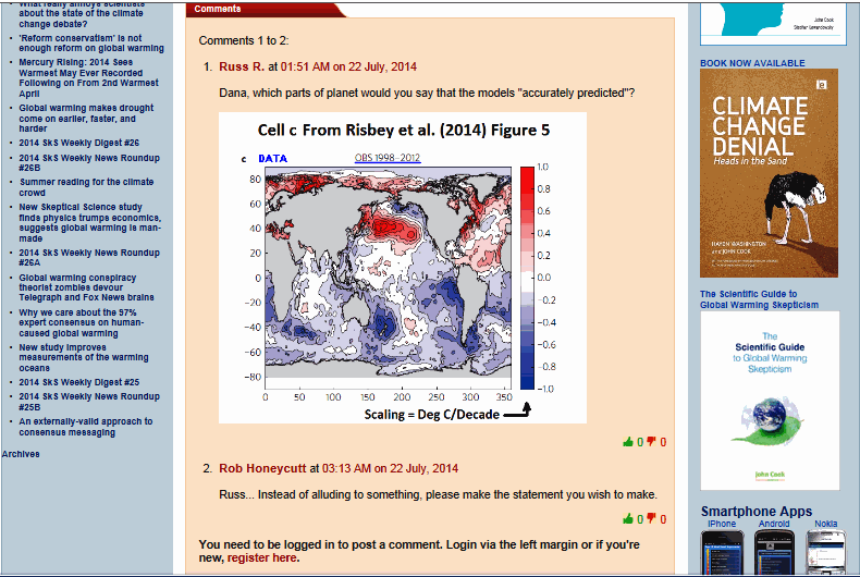
As noted earlier, I’ve been through the paper a number of times, and I cannot find where they listed which models were selected as “best” and “worst”. They illustrated those “best” and “worst” modeled sea surface temperature trends in cells a and b of their Figure 5. See the full Figure 5 from Risbey et al (2014) here. They also illustrated in cell c the observed sea surface temperature warming and cooling trends during the hiatus period of 1998 to 2012. About their Figure 5, they write, where the “in phase” models are the “best” models and “least in phase” models are the “worst” models (my boldface):
The composite pattern of spatial 15-year trends in the selection of models in/out of phase with ENSO regime is shown for the 1998-2012 period in Fig. 5. The models in phase with ENSO (Fig. 5a) exhibit a PDO-like pattern of cooling in the eastern Pacific, whereas the models least in phase (Fig. 5b) show more uniform El Niño-like warming in the Pacific. The set of models in phase with ENSO produce a spatial trend pattern broadly consistent with observations (Fig. 5c) over the period. This result is in contrast to the full CMIP5 multi-model ensemble spatial trends, which exhibit broad warming26 and cannot reveal the PDO-like structure of the in-phase model trend.
Let’s rephrase that. According to Risbey et al (2014), the “best” 4 of their cherry-picked (unidentified) CMIP5 climate models simulate a PDO-like pattern during the hiatus period and the trends of those models are also “broadly consistent” with the observed spatial patterns throughout the rest of the global oceans. If you’re wondering how I came to the conclusion that Risbey et al (2014) were discussing the global oceans too, refer to the second boldfaced sentence in the above quote. Figure 5c presents the trends for all of the global oceans, not just the extratropical North Pacific or the Pacific as a whole.
We’re going to concentrate on the observations and the “best” models in the rest of this section. There’s no reason to look at the models that are lousier than the “best” models, because the “best” models are actually pretty bad.
That is, to totally contradict the claims made, there are no similarities between the spatial patterns in the maps of observed and modeled trends that were presented by Risbey et al (2014)—no similarities whatsoever. See Animation 1, which compares trend maps for the observations and “best” models, from their Figure 5, for the period of 1998 to 2012.
Animation 1
Again, those are the trends for the observations and the models Risbey et al (2014) selected as being “best”. I will admit “broadly consistent” is a vague phrase, but the spatial patterns of the model trends have no similarities with observations, not even the slightest resemblance, so “broadly consistent” does not seem to be an accurate representation of the capabilities of the “best” models.
A further breakdown follows. I normally wouldn’t go into this much detail, but the abstract does close with “spatial trend patterns.” So I suspect that science reporters for newspapers, magazines and blogs are going to be yakking about how well the selected “best” models simulate the spatial patterns of sea surface temperature warming and cooling trends during the hiatus.
My Figure 1 is cell c from their Figure 5. It presents the observed sea surface trends during the hiatus period of 1998-2012. I’ve highlighted 2 regions. At the top, I’ve highlighted the extratropical North Pacific. The Pacific Decadal Oscillation index is derived from the sea surface temperature anomalies in that region, and the Pacific Decadal Oscillation data refers to that region only. See the JISAO PDO webpage here. JISAO writes (my boldface):
Updated standardized values for the PDO index, derived as the leading PC of monthly SST anomalies in the North Pacific Ocean, poleward of 20N.
The spatial pattern of the observed trends in the extratropical North Pacific agrees with our understanding of the “cool phase” of the Pacific Decadal Oscillation (PDO). Sea surface temperatures of the real world in the extratropical North Pacific cooled along the west coast of North America from 1998 to 2012. That cooling was countered by the ENSO-related warming of the sea surface temperatures in the western and central extratropical North Pacific, with the greatest warming taking place in the region east of Japan called the Kuroshio-Oyashio Extension. (See the post The ENSO-Related Variations In Kuroshio-Oyashio Extension (KOE) SST Anomalies And Their Impact On Northern Hemisphere Temperatures.) Because the Kuroshio-Oyashio Extension dominates the “PDO pattern” (even though it’s of the opposite sign; i.e. it shows warming while the east shows cooling during a “cool” PDO mode), the Kuroshio-Oyashio Extension is where readers should focus their attention when there is a discussion of the PDO pattern.
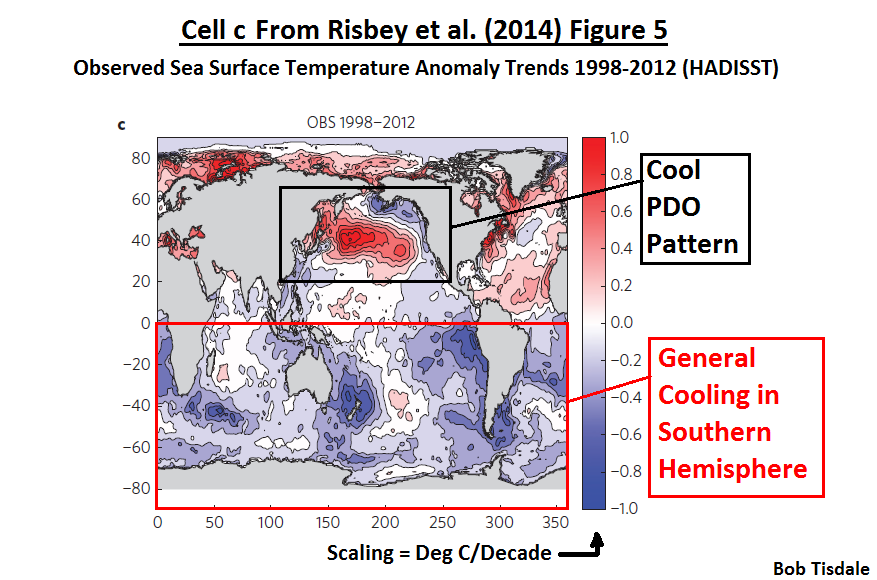
Figure 1
The second “region” highlighted in Figure 1 is the Southern Hemisphere. According to the trend map presented by Risbey et al (2014), real-world sea surface temperatures throughout the Southern Hemisphere (based on HADISST data) cooled between 1998 and 2012. That’s a lot of cool blue trend in the Southern Hemisphere.
I’ve highlighted the same two regions in Figure 2, which presents the composite of the sea surface temperature trends from the 4 (unidentified) “best” climate models. A “cool” PDO pattern does not exist in the extratropical North Pacific of the virtual world of the climate models, and the models show an overall warming of the sea surfaces in the South Pacific and the entire Southern Hemisphere, where the observations showed cooling. If you’re having trouble seeing the difference, refer again to Animation 1.

Figure 2
The models performed no better in the North Atlantic. The virtual-reality world of the models showed cooling in the northern portion of the tropical North Atlantic and they showed cooling south of Greenland, which are places where warming was observed in the real world from 1998 to 2012. See Figures 3 and 4. And if need be, refer to Animation 1 once again.
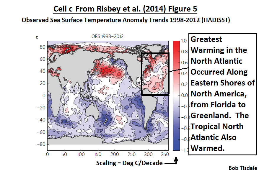
Figure 3
# # #
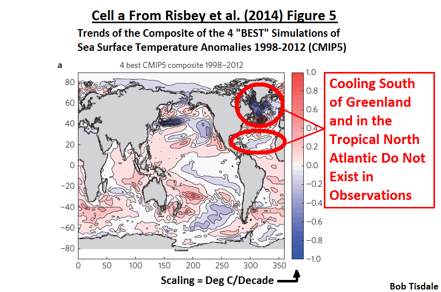
Figure 4
The tropical Pacific is critical to Risbey et al (2014), because El Niño and La Niña events take place there. Yet the models that were selected and presented as “best” by Risbey et al (2014) cannot simulate the observed sea surface temperature trends in the real-world tropical Pacific either. Refer to Figures 5 and 6…and Animation 1 again if you need.
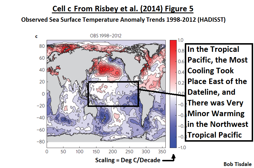
Figure 5
# # #
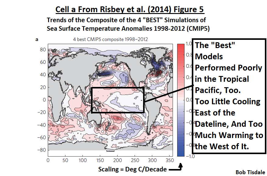
Figure 6
One last ocean basin to compare: the Arctic Ocean. The real-world observations, Figure 7, show a significant warming of the surface of the Arctic Ocean, and that warming is associated with the sea ice loss. The “best” models, of course, shown in Figure 8 do not indicate a similar warming in their number-crunched Arctic Oceans. The differences between the observations and the “best” models stand out like a handful of sore thumbs in Animation 1.

Figure 7
# # #
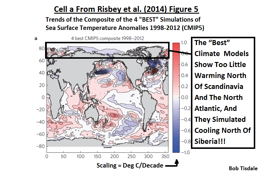
Figure 8
Because the CMIP5 climate models cannot simulate that warming in the Arctic and the loss of sea ice there, Stroeve et al. (2012) “Trends in Arctic sea ice extent from CMIP5, CMIP3 and Observations” [paywalled] noted that the model failures there was an indication the loss of sea ice occurred naturally, the result of “internal climate variability”. The abstract of Stroeve et al. (2012) reads (myboldface):
The rapid retreat and thinning of the Arctic sea ice cover over the past several decades is one of the most striking manifestations of global climate change. Previous research revealed that the observed downward trend in September ice extent exceeded simulated trends from most models participating in the World Climate Research Programme Coupled Model Intercomparison Project Phase 3 (CMIP3). We show here that as a group, simulated trends from the models contributing to CMIP5 are more consistent with observations over the satellite era(1979–2011). Trends from most ensemble members and modelsnevertheless remain smaller than the observed value. Pointing to strongimpacts of internal climate variability, 16% of the ensemble member trendsover the satellite era are statistically indistinguishable from zero. Resultsfrom the CMIP5 models do not appear to have appreciably reduceduncertainty as to when a seasonally ice-free Arctic Ocean will be realized.
WHY CLIMATE MODELS NEED TO SIMULATE SEA SURFACE TEMPERATURE PATTERNS
If you’re new to discussions of global warming and climate change, you may be wondering why climate models must be able to simulate the observed spatial patterns of the warming and cooling of ocean surfaces. The spatial patterns of sea surface temperatures throughout the global oceans are one of the primary factors that determine where land surfaces warm and cool and where precipitation occurs. If climate models should happen to create the proper spatial patterns of precipitation and of warming and cooling on land, without properly simulating sea surface temperature spatial patterns, then the models’ success on land is by chance, not skill.
Further, because climate models can’t simulate where, when, why and how the ocean surfaces warm and cool around the globe, they can’t properly simulate land surface temperatures or precipitation. And if they can’t simulate land surface temperatures or precipitation, what value do they have? Quick answer: No value. Climate models are not yet fit for their intended purposes.
Keep in mind, in our discussion of the Risbey et al. Figure 5, we’ve been looking at the models (about 10% of the models in the CMIP5 archive) that have been characterized as “best”, and those “best” models performed horrendously.
INTERESTING CHARACTERIZATIONS OF FORECASTS AND PROJECTIONS
In the second paragraph of the text of Risbey et al. (2014), they write (my boldface):
A weather forecast attempts to account for the growth of particular synoptic eddies and is said to have lost skill when model eddies no longer correspond one to one with those in the real world. Similarly, a climate forecast of seasonal or decadal climate attempts to account for the growth of disturbances on the timescale of those forecasts. This means that the model must be initialized to the current state of the coupled ocean-atmosphere system and the perturbations in the model ensemble must track the growth of El Niño/Southern Oscillation2,3 (ENSO) and other subsurface disturbances4 driving decadal variation. Once the coupled climate model no longer keeps track of the current phase of modes such as ENSO, it has lost forecast skill for seasonal to decadal timescales. The model can still simulate the statistical properties of climate features from this point, but that then becomes a projection, not a forecast.
If the models have lost their “forecast skill for seasonal and decadal timescales”, they also lost their forecast skill for multidecadal timescales and century-long timescales.
The fact that climate models were not initialized to match any state of the past climate came to light back in 2007 with Kevin Trenberth’s blog post Predictions of Climate at Nature.com’s ClimateFeedback. I can still recall the early comments generated by Trenberth’s blog post. For examples, see Roger Pielke Sr’s blog posts here and here and the comments on the threads at ClimateAudit here and here. That blog post from Trenberth is still being referenced in blog posts (this one included). In order for climate models to have any value, papers like Risbey et al (2014) are now saying that climate models “must be initialized to the current state of the coupled ocean-atmosphere system and the perturbations in the model ensemble must track the growth of El Niño/Southern Oscillation.” But skeptics have been saying this for years.
Let’s rephrase the above boldfaced quote from Risbey et al (2014). It does a good job of explaining the differences between “climate forecasts” (which many persons believe they’ve gotten so far from the climate science community) and the climate projections (which we’re presently getting from the climate science community). Because climate models cannot simulate naturally occurring coupled ocean-atmosphere processes like ENSO and the Atlantic Multidecadal Oscillation, and because the models are not “in-phase” with the real world, climate models are not providing forecasts of future climate…they are only providing out-of-phase projections of a future world that have no basis in the real world.
Further, what Risbey et al. (2014) failed to acknowledge is that the current hiatus could very well last for another few decades, and then, after another multidecadal period of warming, we might expect yet another multidecadal warming hiatus—cycling back and forth between warming and hiatus on into the future. Of course, the IPCC does not factor those multidecadal hiatus periods into their projections of future climate. We discussed and illustrated this in the post Will their Failure to Properly Simulate Multidecadal Variations In Surface Temperatures Be the Downfall of the IPCC?
Why don’t climate models simulate natural variability in-phase with multidecadal variations exhibited in observations? There are numerous reasons: First, climate models cannot simulate the naturally occurring processes that cause multidecadal variations in global surface temperatures. Second, the models are not initialized in an effort to try to match the multidecadal variations in global surface temperatures. It would be a fool’s errand anyway, because the models can’t simulate the basic ocean-atmosphere processes that cause those multidecadal variations. Third, if climate models were capable of simulating multidecadal variations as they occurred in the real world—their timing, magnitude and duration—and if the models were to allowed to produce those multidecadal variations on into the future, then the future in-phase forecasts of global warming (different from the out-of-phase projections that are currently provided) would be reduced significantly, possibly by half. (Always keep in mind that climate models were tuned to a multidecadal upswing in global surface temperatures—a period when the warming of global surface temperatures temporarily accelerated (the term used by Risbey et al.) due to naturally occurring ocean atmosphere processes associated with ENSO and the Atlantic Multidecadal Oscillation.) Fourth, if the in-phase forecasts of global warming were half of the earlier out-of-phase projections, the assumed threats of future global warming-related catastrophes would disappear…and so would funding for climate model-based research. The climate science community would be cutting their own throats if they were to produce in-phase forecasts of future global warming, and they are not likely to do that anytime soon.
A GREAT ILLUSTRATION OF HOW POORLY CLIMATE MODELS SIMULATE THE PAST
My Figure 9 is Figure 2 from Risbey et al. (2014). I don’t think the authors intended this, but that illustration clearly shows how poorly climate models simulate global surface temperatures since the late 1800s. Keep in mind while viewing that graph that it is showing 15-year trends (not temperature anomalies) and that the units of the y-axis is deg K/decade.
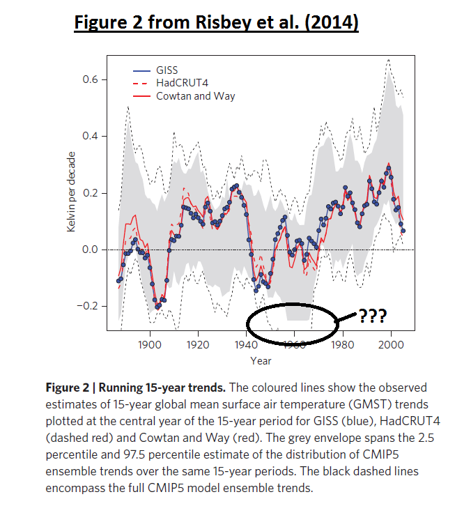
Figure 9
Risbey et al. (2014) describe their Figure 2 as (my boldface):
To see how representative the two 15-year periods in Fig. 1 are of the models’ ability to simulate 15-year temperature trends we need to test many more 15-year periods. Using data from CMIP5 models and observations for the period 1880_2012, we have calculated sliding 15-year trends in observations and models over all 15-year periods in this interval (Fig. 2). The 2.5-97.5 percentile envelope of model 15-year trends (grey) envelops within it the observed trends for almost all 15-year periods for each of the observational data sets. There are several periods when the observed 15-year trend is in the warm tail of the model trend envelope (~1925, 1935, 1955), and several periods where it is in the cold tail of the model envelope (~1890, 1905, 1945, 1970, 2005). In other words, the recent `hiatus’ centred about 2005 (1998-2012) is not exceptional in context. One expects the observed trend estimates in Fig. 2 to bounce about within the model trend envelope in response to variations in the phase of processes governing ocean heat uptake rates, as they do.
While the recent hiatus may not be “exceptional” in that context, it was obviously not anticipated by the vast majority of the climate models. And if history repeats itself, and there’s no reason to believe it won’t, the slowdown in warming could very well last for another few decades.
I really enjoyed the opening clause of the last sentence: “One expects the observed trend estimates in Fig. 2 to bounce about within the model trend envelope…” Really? Apparently, climate scientists have very low expectations of their models.
Referring to their Figure 2, the climate models clearly underestimated the early 20th Century warming, from about 1910 to the early 1940s. The models then clearly missed the cooling that took place in the 1940s but then overestimated the cooling in the 1950s and 60s…so much so that Risbey et al. (2014) decided to erase the full extent of the modeled cooling rates during that period by limiting the range of the y-axis in the graph. (This time climate scientists are hiding the decline in the models.) Then there’s the recent warming period. There’s one reason and one reason only why the models appear to perform well during the recent warming period, seeming to run along the mid-range of the model spread from about 1970 to the late 1990s. And that reason is, the models were tuned to that period. Now, since the late 1990s, the models are once again diverging from the data, because they are not in-phase with the real world.
Will surface temperatures repeat the “cycle” of warming and hiatus/cooling that exists in the data? There’s no reason to believe they will not. Do the climate models simulate any additional multidecadal variability in the future? See Figure 10. Apparently not.
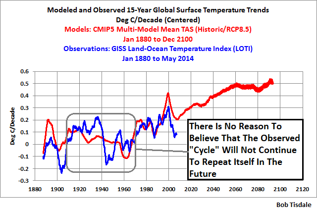
Figure 10
My Figure 10 is similar to Figure 2 from Risbey et al. (2014). For the model simulations of global surface temperatures, I’ve presented the 15-year trends (centered) of the multi-model ensemble-member mean (not the spread) of the historic and RCP8.5 (worst case) forcings (which were also used by Risbey et al.). For the observations, I’ve included the 15-year trends of the GISS Land-Ocean Temperature Index data, which is one of the datasets presented by Risbey et al. (2014). The data and model outputs are available from the KNMI Climate Explorer. The GISS data are included under Monthly Observations and the model outputs are listed as “TAS” on the Monthly CMIP5 scenario runs webpage.
It quite easy to see two things: (1) the modelers did not expect the current hiatus, and (2) they do not anticipate any additional multidecadal variations in global surface temperatures.
Note: If you’re having trouble visualizing what I’m referring to as “cycles of warming and histus/cooling” in Figure 8, refer to the illustration here of Northern Hemisphere temperature anomalies from the post Will their Failure to Properly Simulate Multidecadal Variations In Surface Temperatures Be the Downfall of the IPCC?
OBVIOUSLY MISSING FROM RISBEY ET AL (2014)
One of the key points of Risbey et al. (2014) was their claim that the selected 4 “best” (unidentified) climate models could simulate the spatial patterns of the warming and cooling trends in sea surface temperatures during the hiatus period. We’ve clearly shown that their claims were unfounded.
It’s also quite obvious that Risbey et al. (2014) failed to present evidence that the “best” climate models could reproduce the spatial patterns of the warming and cooling rates in global sea surface temperatures during the warming period that preceded the hiatus. They presented histograms of the modeled and observed trends for the 15-year warming period (1984-1998) before the 15-year hiatus period in cell b of their Figure 1 (not shown in this post). So, obviously, that period was important to them. Yet they did not present how well or poorly the “best” models simulated the spatial trends in sea surface temperatures for the important 15-year period of 1984-1998. If the models had performed well, I suspect Risbey et al. (2014) would have been more than happy to present those modeled and observed spatial patterns.
My Figure 11 shows the observed warming and cooling rates in global sea surface temperatures from 1984 to 1998, using the HADISST dataset, which is the sea surface temperature dataset used by Risbey et al. (2014). There is a clear El Niño-related warming in the eastern tropical Pacific. The warming of the Pacific along the west coasts of the Americas also appears to be El Niño-related, a response to coastally trapped Kelvin waves from the strong El Niño events of 1986/87/88 and 1997/98. (See Figure 8 from Trenberth et al. (2002).) The warming of the North Pacific along the east coast of Asia is very similar to the initial warming there in response to the 1997/98 El Niño. (See the animation here which is Animation 6-1 from my ebook Who Turned on the Heat?) And the warming pattern in the tropical North Atlantic is similar to the lagged response of sea surface temperatures (through teleconnections) in response to El Niño events. (Refer again to Figure 8 from Trenberth et al. (2002), specifically the correlation maps with the +4-month lag.)
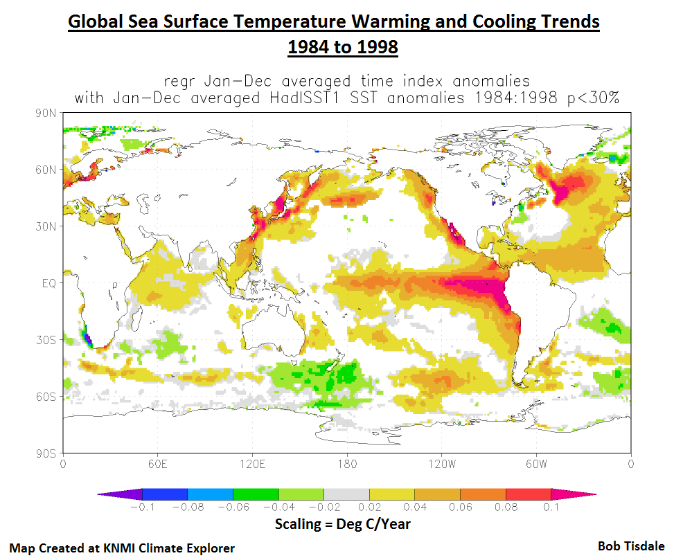
Figure 11
Climate models do not properly simulate ENSO processes or teleconnections, so it really should come as no surprise that Risbey et al. (2014) failed to provide an illustration that should have been considered vital to their paper.
The other factor obviously missing, as discussed in the next section, was the modeled increases in ocean heat uptake. Ocean heat uptake is mentioned numerous times throughout Risbey et al (2014). It would have been in the best interest of Risbey et al. (2014) to show that the “best” models created the alleged increase in ocean heat uptake during the hiatus periods. Oddly, they chose not to illustrate that important factor.
OCEAN HEAT UPTAKE
Risbey et al (2014) used the term “ocean heat uptake” 11 times throughout their paper. The significance of “ocean heat uptake” to the climate science community is that, during periods when the Earth’s surfaces stop warming or the warming slows (as has happened recently), ocean heat uptake is (theoretically) supposed to increase. Yet Risbey et al (2014) failed to illustrate ocean heat uptake with data or models even once. The term “ocean heat uptake” even appeared in one of the earlier quotes from the paper. Here’s that quote again (my boldface):
To see how representative the two 15-year periods in Fig. 1 are of the models’ ability to simulate 15-year temperature trends we need to test many more 15-year periods. Using data from CMIP5 models and observations for the period 1880_2012, we have calculated sliding 15-year trends in observations and models over all 15-year periods in this interval (Fig. 2). The 2.5-97.5 percentile envelope of model 15-year trends (grey) envelops within it the observed trends for almost all 15-year periods for each of the observational data sets. There are several periods when the observed 15-year trend is in the warm tail of the model trend envelope (~1925, 1935, 1955), and several periods where it is in the cold tail of the model envelope (~1890, 1905, 1945, 1970, 2005). In other words, the recent `hiatus’ centred about 2005 (1998-2012) is not exceptional in context. One expects the observed trend estimates in Fig. 2 to bounce about within the model trend envelope in response to variations in the phase of processes governing ocean heat uptake rates, as they do.
Risbey et al. (2014) are making a grand assumption with that statement. There is insufficient subsurface ocean temperature data, for the depths of 0-2000 meters, before the early-2000s, upon which they can base those claims. The subsurface temperatures of the global oceans were not sampled fully (or as best they can be sampled) to depths of 2000 meters before the ARGO era, and the ARGO floats were not deployed until the early 2000s, with near-to-complete coverage around 2003. Even the IPCC acknowledges in AR5 the lack of sampling of subsurface ocean temperatures before ARGO. See the post AMAZING: The IPCC May Have Provided Realistic Presentations of Ocean Heat Content Source Data.
Additionally, ARGO float-based data do not even support the assumption that ocean heat uptake increased in the Pacific during the hiatus period. That is, if the recent domination of La Niña events were, in fact, causing an increase in ocean heat uptake, we would expect to find an increase in the subsurface temperatures of the Pacific Ocean to depths of 2000 meters over the last 11 years. Why in the Pacific? Because El Niño and La Niña events take place there. Yet the NODC vertically average temperature data (which are adjusted for ARGO cool biases) from 2003 to 2013 show little warming in the Pacific Ocean…or in the North Atlantic for that matter. See Figure 12.
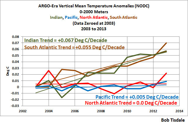
Figure 12
It sure doesn’t look like the dominance of La Niña events during the hiatus period has caused any ocean heat uptake in the Pacific over the past 11 years. Subsurface ocean warming occurred only in the South Atlantic and Indian Oceans. Now, consider that manmade greenhouse gases including carbon dioxide are said to be well mixed, meaning they are pretty well evenly distributed around the globe. It’s difficult to imagine how a well-mixed greenhouse gas like manmade carbon dioxide caused the South Atlantic and Indian Oceans to warm to depths of 2000 meters, while having no impact on the North Atlantic or the largest ocean basin on this planet, the Pacific.
REFERENCE NINO3.4 DATA
For those interested, as a reference for the discussion of Figure 5 from Risbey et al. 2014), my Figure 13 presents the monthly HADISST-based NINO3.4 region sea surface temperature anomalies for the period of January 1998 to December 2012, which are the dataset and time period used by Risbey et al for their Figure 5, and the NINO3.4 region data and model outputs were the bases for their model selection. The UKMO uses the base period of 1961-1990 for their HADISST data, so I used those base years for anomalies. The period-average temperature anomaly (not shown) is slightly negative, at -0.11 Deg C, indicating there was a slight dominance of La Niña events then. The linear trend of the data is basically flat at -0.006 deg C/decade.
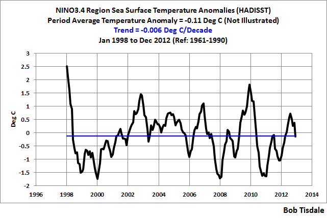
Figure 13
SPOTLIGHT ON CLIMATE MODEL FAILINGS
Let’s return to the abstract again. It includes:
We present a more appropriate test of models where only those models with natural variability (represented by El Niño/Southern Oscillation) largely in phase with observations are selected from multi-model ensembles for comparison with observations. These tests show that climate models have provided good estimates of 15-year trends, including for recent periods and for Pacific spatial trend patterns.
What they’ve said indirectly, but failed to expand on, is:
- IF (big if) climate models could simulate the ocean-atmosphere processes associated with El Niño events, which they can’t, and…
- IF (big if) climate models could simulate the ocean-atmosphere processes associated with longer-term coupled ocean atmosphere processes like the Atlantic Multidecadal Oscillation, another process they can’t simulate, and…
- IF (big if) climate models could simulate the decadal and multidecadal variations of those processes in-phase with the real world, which they can’t because they can’t simulate the basic processes…
…then climate models would have a better chance of being able to simulate Earth’s climate.
Climate modelers have been attempting to simulate Earth’s climate for decades, and climate models still cannot simulate those well-known global warming- and climate change-related factors. In order to overcome those shortcomings of monstrous proportions, the modelers would first have to be able to simulate the coupled ocean-atmosphere processes associated with ENSO and the Atlantic Multidecadal Oscillation…and with teleconnections. Then, as soon as the models have conquered those processes, the climate modelers would have to find a way to place those chaotically occurring processes in phase with the real world.
As a taxpayer, you should ask the government representatives that fund climate science two very simple questions. After multiple decades and tens of billions of dollars invested in global warming research:
- why aren’t climate models able to simulate natural processes that can cause global warming or stop it? And,
- why aren’t climate models in-phase with the naturally occurring multidecadal variations in real world climate?
We already know the answers, but it would be good to ask.
THE TWO UNEXPECTED AUTHORS
I suspect that Risbey et al (2014) will get lots of coverage based solely on two of the authors: Stephan Lewandowsky and Naomi Oreskes.
Naomi Oreskes is an outspoken activist member of the climate science community. She has recently been known for her work in the history of climate science. At one time, she was an Adjunct Professor of Geosciences at the Scripps Institution of Oceanography. See Naomi’s Harvard University webpage here. And she has co-authored at least two papers in the past about numerical model validation.
Stephan Lewandowsky is a very controversial Professor of Psychology at the University of Bristol. How controversial is he? He has his own category at WattsUpWithThat, and at ClimateAudit, and there are numerous posts about his recent work at a multitude of other blogs. So why is a professor of psychology involved in a paper about ENSO and climate models? He and lead author James Risbey gave birth to the idea for the paper. See the “Author contributions” at the end of the Risbey et al. (my boldface):
J.S.R. and S.L. conceived the study and initial experimental design. All authors contributed to experiment design and interpretation. S.L. provided analysis of models and observations. C.L. and D.P.M. analysed Niño3.4 in models. J.S.R. wrote the paper and all authors edited the text.
The only parts of the paper that Stephan Lewandowsky was not involved in were writing it and the analysis of NINO3.4 sea surface temperature data in the models. But, and this is extremely curious, psychology professor Stephan Lewandowsky was solely responsible for the “analysis of models and observations”. I’ll let you comment on that.
CLOSING
The last sentence of the abstract of Risbey et al. (2014) clearly identifies the intent of the paper:
These tests show that climate models have provided good estimates of 15-year trends, including for recent periods and for Pacific spatial trend patterns.
Risbey et al. (2014) took 18 of the 38 climate models from the CMIP5 archive, then whittled those 18 down to the 4 “best” models for their trends presentation in Figure 5. In other words, they’ve dismissed 89% of the models. That’s not really too surprising. von Storch et al. (2013) “Can Climate Models Explain the Recent Stagnation in Global Warming?” found:
However, for the 15-year trend interval corresponding to the latest observation period 1998-2012, only 2% of the 62 CMIP5 and less than 1% of the 189 CMIP3 trend computations are as low as or lower than the observed trend. Applying the standard 5% statistical critical value, we conclude that the model projections are inconsistent with the recent observed global warming over the period 1998-2012.
Then again, Risbey et al. (2014) had different criteria than Von Storch et al. (2013).
Risbey et al. (2014) also failed to deliver on their claim that their tests showed “that climate models have provided good estimates of 15-year trends, including for recent periods and for Pacific spatial trend patterns.” And their evaluation of climate model simulations conveniently ignored the fact that climate models do not properly simulate ENSO processes, which basically means the fundamental overall design and intent of the paper was fatally flawed.
Some readers may believe Risbey et al. (2014) should be dismissed as a failed attempt at misdirection—please disregard those bad models from the CMIP5 archive and only pay attention to the “best” models. But Risbey et al. (2014) have been quite successful at clarifying a few very important points. They’ve shown that climate models must be able to simulate naturally occurring coupled ocean-atmosphere processes, like associated with El Niño and La Niña events and with the Atlantic Multidecadal Oscillation, and the models must be able to simulate those naturally occurring processes in phase with the real world, if climate models are to have any value. And they’ve shown quite clearly that, until climate models are able to simulate naturally occurring processes in phase with nature, forecasts/projections of future climate are simply computer-generated conjecture with no basis in the real world…in other words, they have no value, no value whatsoever.
Simply put, Risbey et al. (2014) has very effectively undermined climate model hindcasts and projections, and the paper has provided lots of fuel for skeptics.
In closing, I would like to thank the authors of Risbey et al. (2014) for presenting their Figure 5. The animation I created from its cells a and c (Animation 1) provides a wonderful and easy-to-understand way to show the failings of the climate-scientist-classified-“best” climate models during the hiatus period. It’s so good I believe I’m going to link it in the introduction of my upcoming ebook. Thanks again.
# # #
UPDATE: The comment by Richard M here is simple but wonderful. Sorry that it did not occur to me so that I could have included something similar at the beginning of the post.
Richard M says: “One could use exactly the same logic and pick the 4 worst models for each 15 year period and claim that cimate [sic] models are never right…”
So what have Risbey et al. (2104) really provided? Nothing of value.
UPDATE 2: Dana Nuccitelli has published a much-anticipated blog post at TheGuardian proclaiming climate models are now accurate due to the cleverness of Bisbey et al (2014). Blogger Russ R. was the first to comment on the cross post at SkepticalScience, and Russ linked my Animation 1 from this post, along with the comment:
Dana, which parts of planet would you say that the models “accurately predicted”?
The gif animation from this post is happily blinking away below that comment. I wasn’t sure how long it would stay there before it was deleted, so I created an animation of two screen caps from the SkS webpage for your enjoyment. Thanks, Russ R.
Note to Rob Honeycutt: I believe Russ asked a very clear question…no alluding involved.


More drivel from the usual suspects.
Anybody who claims that a computer
gamemodel can predict the future state of an effectively infinite non-linear chaotic system driven by an unknown number of feedbacks – of which in some cases we cannot even agree on the sign – that is subject to extreme sensitivity to initial conditions is either a fool or a computer salesman.Ironically, it was Edward Lorenz, a climatologist, who was the first to point this out.
Further, given the “pause” and that the water vapour feedback which is absolutely essential to the whole AGW alarmism industry has stubbornly refused to put in an appearance – in fact Solomon et al showed that atmospheric water vapour had declined by 10% in the first decade of the 21st century – I’m surprised anyone bothers churning out such nonsense an longer.
I’m even more amazed that anyone takes them seriously!
This has made the Guardian
http://www.theguardian.com/environment/climate-consensus-97-per-cent/2014/jul/21/realistic-climate-models-accurately-predicted-global-warming
Check out the first paragraph.
Thanks, mwhite. Propaganda, plain and simple.
Regards
“These tests show that climate models have provided good estimates of 15-year trends, including for recent periods and for Pacific spatial trend patterns.”
In my weather forecast verification work, we use a highly complex and controversial concept set of skill scores that attempted to capture “Forecast minus Observed”.
If I show the “forecast vs observed” graphs of almost all climate models to third graders, the conclusion is obvious. A consensus of 97% third graders agree that the models “busted big time”.
0% of third graders conclude that “It’s happening faster than we thought”
But, as the authors point out, maybe “forecast minus observed” is not an important performance metric.
Thanks, Mary Brown.
I like to read the guardian (I’m a liberal libertarian and I prefer to read left wing papers, Bloomberg and all sorts of crazy blogs), so I read the article they just wrote about this paper. I left this comment a few minutes ago….
“I read the article and the original abstract. I consider the paper’s main theme (that picking models “in phase” with climate cycles out of a model ensemble is a proof of their validity) to be flawed. I suppose the main author and co author didn’t catch this problem.
This tells me there’s a very serious problem with the Nature Inc. family of publications. The editorial quality is way down at Scientific American. Interestingly, I get both the English and Spanish versions, and I sense the lack of quality is much more pronounced in English. This tells me it’s the editors.
As for Nature, my sister and her husband work in biomedical research in the Boston area, they tell me they agree there’s a problem in the biomedical field as well. Too much emphasis on publishing without having solid work behind it. And my sister had to make a full complaint about researchers faking lab notebooks because they had so much pressure to publish something. It can get awful.
To show you I’m not just whining about one single area, I also noticed a decay in the engineering society publications. We get a lot of papers which seem to be intended to market the authors and provide nothing to chew on. Maybe it’s a 21st century effect?
Anyway, I expect this particular paper will be quite controversial. If the abstract is representative then I’m not too impressed.”
I guess I rambled a bit, but my main worry was the actual lack of quality I’m seeing in both scientific and engineering papers.
Thanks, Bob. Reading, analyzing and commenting this paper must have taken a strong stomach.
Pingback: New Climate Model Introduced | Bob Tisdale – Climate Observations
Pingback: New Climate Model Introduced, now with knobs! | Watts Up With That?
“I’ve read and reread Risbey et al. (2014) a number of times and I can’t find where they identify the “best” 4 and “worst” 4 climate models presented in their Figure 5.”
It doesn’t matter what those 4 models are — it is only by chance that their Nino3.4 anomalies aligned closely with the actual Nino3.4 anomalies They didn’t have any special techniques, or any special predictive value; it’ s random.
“I read the article and the original abstract. I consider the paper’s main theme (that picking models “in phase” with climate cycles out of a model ensemble is a proof of their validity) to be flawed.”
That is not at all what the paper claims. It doesn’t claim any particular model has value above any other; only that those models that, by chance, had their Nino3.4 values close to what actually happened, show more pause-like 15-year trends.
“If I show the “forecast vs observed” graphs of almost all climate models to third graders, the conclusion is obvious.”
Climate models don’t do forecasts!!! How often does this need to be repeated?
Climate models solve a boundary value problem, not an initial value problem. Their initial state is not an actual initial state, especially with regard to ENSOs — they are not initialized using observations. Weather models are. They can be initialized with any mean value, because they are calculating the equilibrium state, not the intermediate states, and certainly not the near-term state. Initializing them with any appropriate values will produce the same equilibrium state, but nto the same decadal-scale state.
“Check out the first paragraph.”
The first paragraph is an accurate description of the science..
Bob Tisdale,
You wrote at WUWT:
“Curiously, though, Risbey et al (2014) are pretty much stating that the trend in NINO3.4 sea surface temperature anomalies for any 15-year period dictate the 15-year trends in surface temperatures.”
Could I ask for your help in calculating the correlation between 15-year NINO3.4 trends and 15-year surface temperature trends?
It’s for the thread over at SkS which is getting increasingly entertaining (especially the moderators comments.)
I refer to this paper as Risibley et al. Can you imagine the sort of person who is a climatologist who actually gets involved with La Lewny and the Oreskes creature?
Fernando Leanme is on the money, methinks. I call it the LPU ( least publishable unit) phenomenon. An LPU is the bitcoin of academia or otherwise the defacto metric by which you are effectively judged and assessed. They puff out the CV and get you noticed by the people who do the funding broking. In essence it is a metric of salesmanship and of course in context it is utterly corrupting and a mechanism for degeneration.
David Appell (@davidappell) says: “It doesn’t matter what those 4 models are— it is only by chance that their Nino3.4 anomalies aligned closely with the actual Nino3.4 anomalies They didn’t have any special techniques, or any special predictive value; it’ s random.”
Of course the relationship between data and modeled NINO3.4 SSTa was accidental. That still does not relieve the authors from supplying information that allows others to verify their results.
Regarding your second and third comments, David, I’ll let their authors reply.
David Appell (@davidappell) replies to mwhite’s comment about Dana Nuccitelli’s opening paragraph at the Guardian: “The first paragraph is an accurate description of the science.”
Actually, it’s not. Dana’s opening paragraph reads, “Predicting global surface temperature changes in the short-term is a challenge for climate models. Temperature changes over periods of a decade or two can be dominated by influences from ocean cycles like El Niño and La Niña. During El Niño phases, the oceans absorb less heat, leaving more to warm the atmosphere, and the opposite is true during a La Niña.”
An ENSO index (NINO3.4 SSTa) correlates very poorly with the NODC’s depth-averaged temperature anomalies for the top 700 meters and 2000 meters, David. We can’t use the NODC OHC data for that analysis, because their ocean heat content data for the top 2000 meters are only available in pentadal form. Luckily, their vertically averaged temperature data are available in annual form.
For the period of 1955 to 2013, the correlation coefficient (0-year lag) for NINO3.4 SSTa (Kaplan SST) and the NODC vertically-averaged temperature data for the depths of 0-2000 meters is -0.14. Horrendous! It gets slightly worse for 0-700 meters, David. For the period of 1955 to 2013, the correlation coefficient (0-year lag) for NINO3.4 SSTa (Kaplan SST) and the NODC vertically-averaged temperature data for the depths of 0-700 meters is -0.12.
The sampling for older subsurface temperature data is terrible, so let’s look at the ARGO era, David. For the period of 2003 to 2013, the correlation coefficient (0-year lag) for NINO3.4 SSTa (Kaplan SST) and the NODC vertically-averaged temperature data for the depths of 0-2000 meters is -0.34. Still pretty awful. And it’s again worse for the depths of 0-700 meters. For the period of 2003 to 2013, the correlation coefficient (0-year lag) for NINO3.4 SSTa (Kaplan SST) and the NODC vertically-averaged temperature data for the depths of 0-700 meters is -0.29.
The correlations get a little better for the ARGO era if we lag the NINO3.4 data by a year, but we’re still talking correlation coefficients in the neighborhood of -0.5.
So data do not support Nuccitelli’s conjecture. Nothing surprising there.
Keep in mind, David, the tropical Pacific may release more heat than normal during an El Niño, but that conveniently overlooks other ocean basins that warm in response to El Niño-caused decreases in evaporation and increases in sunlight, and the fact that wind patterns (sea level pressures) in those ocean basins also impact ocean heat uptake.
Thanks for stopping by, David.
Russ R. says: “Could I ask for your help in calculating the correlation between 15-year NINO3.4 trends and 15-year surface temperature trends?”
Luckily, I had prepared it for this post but I elected not to include it because I didn’t think it really added to the discussion. But here you are:

There is basically no correlation between the two.
Sounds like you’re having fun over there. Who said the 15-year trends of the two datasets correlated well?
Pingback: DoubleThink – The ‘wonder’ of Climate Models | the WeatherAction Blog
Thanks Bob,
I was mistaken in believing the two were correlated.
Appreciate your setting me straight.
The bogus science will never end. I’m very grateful to Bob Tisdale and others for the incredible amount of work they’re doing analyzing the constant influx of fraudulent research.
We know that AGW is a political/economic scam disguised as environmental concern. We need to focus on the fact that fraud and lousy science are a diversion; AGW-alarmists support AGW because they believe it’s “green”, as scientists, we should realize that our attention is intentionally diverted from the NWO fascist agenda by “bogus science”. Bogus science is equivalent to green. Environmentalists with no physical science knowledge and physical scientists who are justifiably outraged by this type of research are ideal segments of the population to manipulate through constant distractions from the big picture.
“That still does not relieve the authors from supplying information that allows others to verify their results.”
You’re free to download the CMIP5 results and do their calculation for yourself. See if you find four models.
I can understand why they didn’t want to name the 4 models — it would give the wrong impression, just like, in fact, your take on it that youi wrote about in your post.
“they support AGW because they believe it’s “green””
I accept most of AGW because physics requires it to happen, and I understand the physics. Maybe you don’t.
“There is basically no correlation between the two.”
Again you show that you don’t understand the paper. The paper doesn’t claim there is a correlation — instead, it looks at models that are accidentally correlated to Nino3.4 (and the correlation is to the model’s Nino3.4 anomalies, not to surface temperatures.)
“An ENSO index (NINO3.4 SSTa) correlates very poorly with the NODC’s depth-averaged temperature anomalies for the top 700 meters and 2000 meters, David.”
That’s exactly the point! They aren’t saying the Nino3.4 index is correlated to surface warming or to ocean warming. They are saying that models that *do* correlate, by random, show more pause-like features than models that don’t.
You don’t seem to have understood this paper at all.
Climate models solve a boundary value problem, not an initial value problem. Their initial state is not an actual initial state, especially with regard to ENSOs — they are not initialized using observations.
Heh. The atmosphere is an unbound system, so what he’s saying is the climate models are… Isn’t that another way of saying they’re useless?
Reblogged this on Tallbloke's Talkshop and commented:
Tremendous post from Bob Tisdale. Lewandowsky strikes (out) again.
Thanks Bob, this is a great post. Lew always offers a rich vein of satirical material. The gift that keeps giving!
David Appell (@davidappell) says: “You’re free to download the CMIP5 results and do their calculation for yourself. See if you find four models.”
David, you’re wasting my time. Take it elsewhere.
Verification is not about being able to find 4 models; it’s about being able to find the same 4 models. And it’s about being able to find the same models Risbey et al presented for each of the 15-year periods. Other than the size of the dots in their illustrations, they did not identify the number of models they used for each of the 15-year periods. BTW, the CMIP5 models are available through the KNMI Climate Explorer, so there’s no need to download the CMIP5 results.
In response to my answer to a question from another blogger, you, David, wrote, “Again you show that you don’t understand the paper. The paper doesn’t claim there is a correlation — instead, it looks at models that are accidentally correlated to Nino3.4 (and the correlation is to the model’s Nino3.4 anomalies, not to surface temperatures.)”
I was answering a question from another blogger on this thread, David. I was not commenting to the paper. So your little rant is baseless. And you continued to waste my time with your next comment.
In response to my comment about ocean warming in the opening paragraph of Nuccitelli’s Guardian article, you, David, wrote “That’s exactly the point! They aren’t saying the Nino3.4 index is correlated to surface warming or to ocean warming. They are saying that models that *do* correlate, by random, show more pause-like features than models that don’t.
“You don’t seem to have understood this paper at all.”
My comment about ocean heat content was not about the paper, David. It was about the opening paragraph of Nuccitelli’s blog post.
Your recent comments highlight problems that you have, David. They are not a problem on my part. It will be very obvious to everyone who visits this thread that you can’t differentiate between my comments on the paper and my comments about other people’s comments on the paper or my answers to questions posed by other bloggers.
You’re wasting my time, David. Take it elsewhere.
Adios.
Do you think this quiet sun period will give us clues to the Maunder and Dalton minimums? Is anyone looking for that specifically?
Anybody who claims that a computer game model can predict the future state of an effectively infinite non-linear chaotic system driven by an unknown number of feedbacks – of which in some cases we cannot even agree on the sign – that is subject to extreme sensitivity to initial conditions is either a fool or a computer salesman.
Quite right. But that is not all. It is not clear that all the required inputs are measured. Let alone included in the models. Of course the measurements of even the known inputs is not accurate enough even if the climate was strictly linear and non-chaotic. Take TSI which is supposed to be measured to 1 part in 1,000 accuracy. But satellites that are observing at the same time do not agree within that margin of error.
So what is done to the reported numbers? Slicing, dicing, and homogenization. Willie Soon called it out. To get some idea of how the space environment affects the measurements and the measuring instruments we would have to launch a series of them of the same design for a few years in a row so that there was significant data overlap. That might not tell us enough. But right now we have next to nothing. Well very little. In addition different types of instruments should also be available to check for design concept flaws.
M Simon says: “Do you think this quiet sun period will give us clues to the Maunder and Dalton minimums? Is anyone looking for that specifically?”
M Simon, sorry to say, but my focus is primarily on the satellite era. And I pay very little attention to anything before the 1900s.
Who studies that? See Dr. Leif Svalgaard’s (solar physicist from Stanford University) comments on pretty much any solar thread at WattsUpWithThat. And if you have any additional questions, Leif is open to solar questions even if they’re slightly off topic. The next solar update at WUWT should be within the next few weeks, maybe sooner. Leif’s also got lots of links to papers, etc, at his website.
http://www.leif.org/research/
Regards
Pingback: PACIFIC OCEAN SST …Time series graphs | CRIKEY !#&@ ...... IT'S THE WEATHER CYCLES
Pingback: WOW! – How Many Fabrications, Misrepresentations, etc., Can One Blogger Roll into One Blog Post? | Bob Tisdale – Climate Observations
Thanks for the reblog and traffic, tallbloke.
Cheers!!!
Bob,
I’m sorry to say but in my opinion Leif is not very impressive. I won’t go into all the details but from what I can tell he is of the opinion that TSI is all that matters and it doesn’t matter. Not very open minded.
Bob Tisdale, a one-man show which puts the established (TM) climate science to shame by pointing to the observed data. Glad you exist, Bob!
M Simon, Leif is very open minded when the arguments are sound. Keep in mind that Leif has decades of rigorous research behind him, and for many years, he’s responded to all of the theories people continue to present.
Bob,
I think David Appell actually has a point when he describes the operational purpose of a climate model:
“Climate models don’t do forecasts!!! How often does this need to be repeated?
Climate models solve a boundary value problem, not an initial value problem. Their initial state is not an actual initial state, especially with regard to ENSOs — they are not initialized using observations. Weather models are. They can be initialized with any mean value, because they are calculating the equilibrium state, not the intermediate states, and certainly not the near-term state. Initializing them with any appropriate values will produce the same equilibrium state, but nto the same decadal-scale state.”
The simple aim of the paper is to show that GCMs, slowly progressing towards their equilibrium state, will not catch intermediate plateaus on the way there because they don’t have it in them to reproduce short term/medium term natural variability (noise, if you will). The underlying claim is that the equilibrium state will be reached at some point, with or without a ‘pause’ or two in between, and that this particular ‘pause’ is caused by the prevailing ENSO phase … which the GCMs can’t and don’t capture.
I think the paper actually makes a logically consistent case in this way, even though I certainly don’t agree with the implication that ENSO is merely noise and the only real driver of recent and future climate is CO2.
But, yes, a lot of words and very little supporting information provided, I agree.
Kristian says: “I think David Appell actually has a point when he describes the operational purpose of a climate model…”
Climate models have to be portrayed that way because climate models cannot simulate natural factors such ENSO and the AMO. If they were capable of simulating those processes, then the models could be initialized to actual conditions with hope of coming close to natural variations. Climate models, as they exist now, provide simulations of a world that have no similarities to the one we inhabit, and as a result they are of little value.
Further, does the public at large know the operational purpose of a climate model is only to portray the possible impacts of manmade greenhouse gases on a world that has no relationship to the real world? No, they do not.
Regards
Bob Tisdale says, July 24, 2014 at 12:10 pm:
“Climate models have to be portrayed that way because climate models cannot simulate natural factors such ENSO and the AMO. If they were capable of simulating those processes, then the models could be initialized to actual conditions with hope of coming close to natural variations. Climate models, as they exist now, provide simulations of a world that have no similarities to the one we inhabit, and as a result they are of little value.
Further, does the public at large know the operational purpose of a climate model is only to portray the possible impacts of manmade greenhouse gases on a world that has no relationship to the real world? No, they do not.”
Couldn’t agree more, Bob 🙂
Kirstan,
The simple aim of the paper is to show that GCMs, slowly progressing towards their equilibrium state, will not catch intermediate plateaus on the way there because they don’t have it in them to reproduce short term/medium term natural variability (noise, if you will).
If they can’t do that reasonably well they can’t model a chaotic system.
But you may have made Bob’s point inadvertently. The job of the “models” is not to model. It is to fool the public. Ah. I see you agree with Bob. Consider this a redundant affirmation of your point and Bob’s.
BTW climate has no equilibrium state. Because it is a chaotic system the best you can do is find its strange attractors. The fact that you think they are trying to reach an equilibrium state – if true – shows just how far off and ignorant the modelers are.
Habibullo Abdussamatov. disagrees with Lief.
Significant climate variations during the past 7.5 millennia indicate that bicentennial quasi-periodic TSI variations define a corresponding cyclic mechanism of climatic changes from global warmings to Little Ice Ages and set the timescales of practically all physical processes taking place in the Sun-Earth system. Quasi-bicentennial cyclic variations of the TSI entering the Earth’s upper atmosphere are the main fundamental cause of corresponding alternations of climate variations.
http://www.oarval.org/ClimateChangeBW.htm
(you have to scroll down a bit)
Also look at this chart that goes with the above:
Figure 1. Variations of both the TSI and solar activity in 1978-2013 and prognoses of these variations to cycles 24-27 until 2045. The arrow indicates the beginning of the new Little Ice Age epoch after the maximum of cycle 24.
The arrow points to 2014.
M Simon says, July 24, 2014 at 2:22 pm:
“Ah. I see you agree with Bob. Consider this a redundant affirmation of your point and Bob’s.”
I very much agree with Bob. I’m just trying to be a devil’s advocate here. To see it from their perspective. And I do in fact think that within that fictitious realm that the models and their modellers have created for themselves, this paper actually makes a sound point.
The bottom line, though, is that what this paper has really accomplished, is to finally prove beyond all doubt (if there ever were any) that the models are purely tuned to ‘CO2 forcing’ as the climate driver. Everything else is considered noise or insignificant. Eventually the temp will go up either way, no matter what happens with natural variability. So why bother with the models at all? Why not just extrapolate the Keeling curve indefinitely into the future and let temps follow that one? Well, that is basically what they do anyway …
The climate models have never been a tool to actually test the validity of the AGW hypothesis (like they should’ve been). They were always only a tool to project temperatures as if the hypothesis had already been tested and found valid.
The warmists wouldn’t know what a ‘circular argument’ is if it bit them in the behind.
Sorry, “… wouldn’t know a ‘circular argument’ if …” Mix-up.
Pingback: June 2014 Global Surface (Land+Ocean) and Lower Troposphere Temperature Anomaly Update | Bob Tisdale – Climate Observations
Pingback: June 2014 Global Surface (Land+Ocean) and Lower Troposphere Temperature Anomaly Update | Watts Up With That?
[SNIP. Off topic.]
papiertigre says:
“Heh. The atmosphere is an unbound system….”
The Earth’s climate system is not unbounded — the primary constraint being energy conservation for the system as a whole:
“Climate modeling is also fundamentally different from weather forecasting. Weather concerns an initial value problem: Given today’s situation, what will tomorrow bring? Weather is chaotic; imperceptible differences in the initial state of the atmosphere lead to radically different conditions in a week or so. Climate is instead a boundary value problem — a statistical description of the mean state and variability of a system, not an individual path through phase space. Current climate models yield stable and nonchaotic climates, which implies that questions regarding the sensitivity of climate to, say, an increase in greenhouse gases are well posed and can be justifiably asked of the models. Conceivably, though, as more components — complicated biological systems and fully dynamic ice-sheets, for example — are incorporated, the range of possible feedbacks will increase, and chaotic climates might ensue.”
http://www.giss.nasa.gov/research/briefs/schmidt_04/
M Simon says:
“If they can’t do that reasonably well they can’t model a chaotic system.”
Climate models don’t try to model a chaotic system — which, of course, no one knows how to do. They calculate equillibrium states, which is relevant because short-term variations like ENSO, PDO, AMO etc, — from observations, we know these tend to average out to about zero in the long-term, so climate models are relevant (and, in any case, the only tool available to project the equilibrium state given any forcing.
But it’s possible there will be a chaotic change to climate that is unforeseen, and the possibility of this goes up as the system’s energy goes up (warming).
M Simon says:
“BTW climate has no equilibrium state. Because it is a chaotic system the best you can do is find its strange attractors.”
Determination of paleoclimates show that the climate system usually does have an equilibrium state — for example, the regularity of recent ice ages, and the warming during the PETM. Chaos seems rare on decadal timescales.
But the climate system certainly can jump into an unforeseen state. This makes our current situation worse, not better.
Bob Tisdale wrote:
“Climate models have to be portrayed that way because climate models cannot simulate natural factors such ENSO and the AMO. If they were capable of simulating those processes, then the models could be initialized to actual conditions with hope of coming close to natural variations.”
Why don’t you show the way in how to predict ENSOs?
Given today’s initial conditions, when will the next ten ENSOs occur, and what will be their magnitudes?
No one knows how to do that, and it’s doubtful we have nearly enough observations of the initial state to do it — ENSO models alone, which do take short-term initial conditions, do only a moderate job at best. There seems to be little-to-no periodicability or patterns that provide a direct determinism of ENSO states — not know, and not into the future.
But since ENSOs average out to about zero over the long-term (several decades+), it suffices to solve the long-term (boundary value) climate problem. In 50 years it won’t matter that ENSOs conspired to produce a 15-yr slowdown of surface temperatures, just as today it doen’t matter that the 1940s-1970s were foreseen. Heat is still being added to the system, and it must manifest somehow.
There was a even deeper slowdown in the mid-1990s:
http://davidappell.blogspot.com/2014/03/the-lesser-of-two-pauses.html
That slowdown was also helped by unpredictable natural variability (Pinatubo). So unless you can also predict volcanic eruptions, especially the big ones, it is again impossible for climate models to predict short-term states. That’s also apparently been a factor in this slowdown:
“Volcanic contribution to decadal changes in tropospheric temperature,”
Benjamin D. Santer, Nature Geoscience 7, 185–189 (2014).
http://www.nature.com/ngeo/journal/v7/n3/full/ngeo2098.html
Bob Tisdale wrote:
“Climate models, as they exist now, provide simulations of a world that have no similarities to the one we inhabit, and as a result they are of little value.”
They provide a simulation to the most realistic future world we can envision — which is not one that will include every ENSO, every volcanic eruption, every exact emission path of aerosols and CO2 and CH4 and every ozone hole. every variation in solar irradiance, etc etc.
But climate models are of great value, because, though imperfect, they are the best tool we have for determing the likely path of today’s climate
Bob Tisdale wrote:
“Further, does the public at large know the operational purpose of a climate model is only to portray the possible impacts of manmade greenhouse gases on a world that has no relationship to the real world? No, they do not.”
And your inaccuracies in portarying models, such as this post, don’t help.
Bob Tisdale wrote:
“You’re wasting my time, David. Take it elsewhere. Adios.”
Yes, I often find such a response from WUWT-like people who don’t appreciate and can’t handle their positions being contested. It is the exact opposite of how science is really done and how scientists really behave.
Bob Tisdale wrote:
“Verification is not about being able to find 4 models; it’s about being able to find the same 4 models.”
Yet again — they aren’t verifying models! They aren’t. Instead, they show that models that happen — by chance — to be aligned with recent ocean states do a better job of projecting the slowdown than do models not in alighnment.
Their paper is not at all about verifying models. Hence the specific models don’t matter, because there is nothing special about them.
Of course, you’re always free to write the authors and ask about the four models. How hard is that?
David Appell (@davidappell) says: “Why don’t you show the way in how to predict ENSOs?”
Nice try at misdirection, David, but it failed. The models can’t simulate the basic processes of ENSO and the AMO. That was my point. Only then can the modelers even hope to be able to simulate the multidecadal variability in each of those processes. Nowhere in my post and comments did I ever say that I expected climate models to replicate every little wiggle, my comments were about multidecadal contributions.
David Appell (@davidappell) says: “But since ENSOs average out to about zero over the long-term (several decades+)…”
More misdirection, David, with misinformation added to spice up your comment. Maybe ENSO averages out to zero in climate models where ENSO is not simulated correctly, but in the real world, David, the processes of ENSO discharge and distributed heat as a result of El Niños and recharge heat (with sunlight) during La Niñas. As such, your comment in nonsensical.
David Appell (@davidappell) says: “They provide a simulation to the most realistic future world we can envision — which is not one that will include every ENSO, every volcanic eruption, every exact emission path of aerosols and CO2 and CH4 and every ozone hole. every variation in solar irradiance, etc etc.”
Thank you for taking my comment out of context, David. The sentence you quoted (and replied to) related to models not being able to simulate basic ENSO and AMO processes. Once again, more misdirection from you.
Apparently you find models that cannot simulate the multidecadal effects of ENSO and the AMO to be credible, when both ENSO and the AMO can naturally contribute to or suppress global warming, and you obviously haven’t grasped the importance of the fact that the models were tuned to a multidecadal naturally occurring upswing in global surface temperatures caused by a dominance of El Niño events and an upswing in the AMO.
David Appell (@davidappell) says: “Yet again — they aren’t verifying models!”
And once again, you’re using misdirection, David. Yet again — my comment was NOT about Risbey et al. verifying models; my comment was about others being able to verify the results of Risbey et al.
David Appell (@davidappell) says: “And your inaccuracies in portarying [sic] models, such as this post, don’t help.”
My portrayal of models in the post was very accurate, David. And your comments on this thread confirmed many of my main points directly or indirectly. People reading this thread can see very plainly that you’re trying (and failing) to downplay the significant role that nature played in the warming we had experienced…something that modelers exclude from their hindcasts and projections. And now that those contributions are no longer there, you, David, are making excuses for the models. Excuses don’t work. Thanks.
David Appell (@davidappell) says: “Yes, I often find such a response from WUWT-like people who don’t appreciate and can’t handle their positions being contested.”
In reality, David, I have no trouble when someone contests my position. But, I have trouble with people such as you, David, taking my comments out of context, and I have trouble with people such as you, David, trying misdirection (and failing in its use), and I have trouble with people such as you, David, trying to misinform, all the while reinforcing the points I made in my post—because I need to respond to your comments, which is a waste of my time. Because you insist on wasting my time, you’re now banned from this thread.
Adios.
Is this a (probably failed) attempt to do some science, or is it just a Séralini (a guaranteed 0% science PR stunt)?
Current climate models yield stable and nonchaotic climates, which implies that questions regarding the sensitivity of climate to, say, an increase in greenhouse gases are well posed….
Well posed is one thing correct is another. Now suppose the coefficients are significantly wrong. And clouds which are very significant…. Even the modelers admit they do not do clouds well.
Well. That sort of thing tends to induce doubt. Or scepticism if you will. Or denial that the models are correct.
Chaos seems rare on decadal timescales.
But the climate system certainly can jump into an unforeseen state. This makes our current situation worse, not better.
The states are not unforseen. It is just the timing of the jumps that is unpredictable. Unless you accord Habibullo Abdussamatov with the ability to predict the coming Dalton like minimum with associated cooling. He says we will see evidence this year.
Australia is having a very cold winter. And North America is having a cool summer. Of course it could just be weather. Time will tell.
====
http://notrickszone.com/2013/12/03/german-scientists-show-climate-driven-by-natural-cycles-global-temperature-to-drop-to-1870-levels-by-2100/
The present “stagnation” of global temperature (Fig. 5) is essentially due to the AMO/PDO: the solar de Vries cycle is presently at its maximum. Around this maximum it changes negligibly. The AMO/PDO is presently beyond its maximum, corresponding to the small decrease of global temperature. Its next minimum will be 2035. The temperature can expected to be then similar to the last AMO/PDO minimum of 1940. Due to the de Vries cycle, the global temperature will drop until 2100 to a value corresponding to the “little ice age” of 1870.
===
It is worse than we thought. But not in the direction predicted by CO2 driven models. Got any spare “change” ?
[Snip! along with the other 3 comments.]
David Appell, if you’re wondering about the snips, I had already replied to your comments about ENSO (a recharge/discharge oscillator does not average out over time), and had you read my last reply in full, you would have noted I had banned you from this thread.
Bob, I’m not surprised you banned me. People like you and AW always do — it’s how you maintain your climate fantasy world..
I know you like to pretend you’re a scientist. You’re not nearly scientifically lcapable enough to pull that off, nor capable of tolerating dissent like scientists do. Insecurity?
You’re welcome to comment at my blog anytime.
Good-bye, David. You continue to waste your time and mine.
Contrary to your statement, I’ve never claimed to be a scientist. In fact, I wouldn’t want to be a climate scientist.
Hang around, though. I’ve got another post coming about Risbey et al. (2014). You won’t like that one either.
Pingback: More on the Lewendowski and Oreskes Co-Authored Paper Risbey et al. (2014) | Bob Tisdale – Climate Observations
Pingback: More on the Lewandowsky and Oreskes Co-Authored Paper Risbey et al. (2014) | Watts Up With That?
Pingback: AOGCM E Temperature Oceaniche: a quando previsioni accurate? | Climatemonitor
I appreciate that this paper is long since dead and buried, but aTTP breathed some life into it over at Climate Audit and it got me to reread it. The key issue that rather got downplayed here and at WUWT was that the 15 year trend in NINO3.4 is most unlikely to have any useful relationship with the status of ENSO over that period. It is far too crude an index (and highly volatile – a model that performs well one year fails the next).
I thought I would investigate an index that looked at the correlation between each model NINO3.4 and the observed index instead. Unfortunately I can’t find a downloadable historic CMIP5 NINO3.4 for each model that would allow its derivation (and constructing the index from the model temp output is beyond my attention span).
Is there a downloadable version around? Presumably Risbey et al. got access to one – I doubt they’d produced the indices themselves.
HAS, I know of no website that lists the NINO3.4 TOS outputs for the CMIP5 models.
The KNMI Climate Explorer is the only website I use for CMIP5 model outputs. If you’re interested in knowing which model you’re dealing with, you’d have to input the coordinates of the NINO3.4 region for each individual model for the variable TOS. Climate Explorer then provides the NINO3.4 output for each of the ensemble members.
And I’ll agree with you that there is likely no relationship between modeled and observed ENSO.