In Honor of the 4th of July, A Few Model-Data Comparisons of Contiguous U.S. Surface Air Temperatures

This post is similar in format to In Honor of Secretary of State John Kerry’s Global Warming Publicity-Founded Visit to Greenland…  As you’ll see, like Greenland, the consensus of the climate models used by the IPCC show that the models do not simulate the surface temperatures for the contiguous United States over any timeframe from 1861 to present. 

INTRODUCTION

We illustrated and discussed the wide ranges of modeled and observed absolute global surface temperatures in the November 2014 post On the Elusive Absolute Global Mean Surface Temperature – A Model-Data Comparison. Not long after came a post at RealClimate of modeled absolute global surface temperatures, authored by Gavin Schmidt, the head of the Goddard Institute of Space Studies (GISS).  Gavin’s post is Absolute temperatures and relative anomalies.  (Please read it in its entirety.  I believe you’ll find it interesting.)  Of course, Gavin Schmidt was downplaying the need for climate models to simulate Earth’s absolute surface temperatures.

In this post about the surface temperatures of the contiguous United States, we’ll present a few examples of why climate modelers need to shift their focus from surface temperature anomalies to absolute surface temperatures.  Why?  In addition to heat waves and cold spells, near-surface air temperatures play roles in model simulations of snow cover, drought, growing seasons, surface evaporation that contributes to rainfall, etc.

In the past, we’ve compared models and data using time-series graphs of temperature anomalies, absolute temperatures and temperature trends, and we’ll continue to provide them in this post.  In this series, we’ve added a new model-data comparison graph:  annual cycles based on the most-recent recent multidecadal period. Don’t worry, that last part will become clearer later in the post.

MODELS AND DATA

We’re using the model-mean of the climate models stored in the CMIP5 (Coupled Model Intercomparison Project Phase 5) archive, with historic forcings through 2005 and RCP8.5 forcings thereafter.  (The individual climate model outputs and model mean are available through the KNMI Climate Explorer.) The CMIP5-archived models were used by the IPCC for their 5^th Assessment Report. The RCP8.5 forcings are the worst-case future scenario.

We’re using the model-mean (the average of the climate model outputs) because the model-mean represents the consensus of the modeling groups for how surface temperatures should warm if they were warmed by the forcings that drive the models. See the post On the Use of the Multi-Model Mean for a further discussion of its use in model-data comparisons.

I’ve used the ocean-masking feature of the KNMI Climate Explorer and the coordinates of 24N-49N, 125W-66W to capture the modeled near-land surface air temperatures of the contiguous United States, roughly the same coordinates used by Berkeley Earth.

Near-surface air temperature observations for the contiguous U.S. are available from the Berkeley Earth website, specifically the contiguous United States data here. While the monthly data are presented in anomaly form (referenced to the period of 1951-1980), Berkeley Earth provides the monthly values of their climatology in absolute terms, which we then simply add to the anomalies of the respective months to determine the absolute monthly values.   Most of the graphs, however, are based on annual average values to reduce the volatility of the data.

The model mean of surface temperatures at the KNMI Climate Explorer starts in 1861 and the Berkeley Earth data end in August 2013, so the annual data in this post run from 1861 to 2012.

ANNUAL NEAR-LAND SURFACE AIR TEMPERATURES – THE CONTIGUOUS UNITED STATES

Figure 1 includes a time-series graph of the modeled and observed annual near-land surface air temperature anomalies for the contiguous U.S. from 1861 to 2012. Other than slightly underestimating the long-term warming trend, at first glance, the models appear to do a reasonable job of simulating the warming (and cooling) of the surfaces of the contiguous United States. But as we’ll see later in the post, the consensus of the models misses the multidecadal warming from the early 1910s through the early 1940s.

Figure 1

Keep in mind, Figure 1 is how climate modelers prefer to present their models, in anomaly form.

Figure 2 gives you an idea of why they prefer to present anomalies. It compares the modeled and observed temperatures on an absolute basis. Not only do the models miss the multidecadal variations in the surface temperatures of the contiguous United States, the consensus of the models is running too cold.  That of course would impact how well the models simulate temperature-related factors like snowfall, drought, crop yields and growing seasons, heat waves, cold spells, etc.

Figure 2

ANNUAL CYCLES

Climate is typically defined as the average conditions over a 30-year period.  The top graph in Figure 3 compares the modeled and observed average annual cycles of the contiguous U.S. surface temperatures for the most recent 30-year period (1983 to 2012). Over that period, data indicate that the average surface temperatures for the contiguous U.S. varied from about +0.0 deg C (+32 deg F) in January to roughly +24.0 deg C (+75 deg F) in July.  On the other hand, the consensus of the models show they are too cool by an average of about 1.4 deg C (2.5 deg F) over the course of a year.

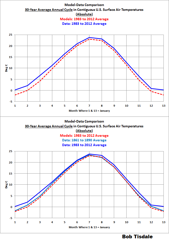
Figure 3

You might be saying to yourself, it’s only a model-data difference of -1.4 deg C, while the annual cycle in surface temperatures for the contiguous U.S. is about 24 deg C.  But let’s include the annual cycle of the observations for the first 30-year period, 1861-1890. See the light-blue curve in the bottom graph in Figure 3. The change in observed temperature from the 30-year period of 1861-1890 to the 30-year period of 1983-2012 is roughly 1.0 deg C, while the model-data difference for the period of 1983-2012 is greater than that at about 1.4 deg C.

THE MODELS ARE PRESENTLY SIMULATING AN UNKNOWN PAST TEMPERATURE-BASED CLIMATE IN THE CONTIGUOUS UNITED STATES, NOT THE CURRENT CLIMATE

Let’s add insult to injury. For the top graph in Figure 4, I’ve smoothed the data and model outputs in absolute form with 30-year running-mean filters, centered on the 15^th year. Again, we’re presenting 30-year averages because climate is typically defined as 30 years of data.  This will help confirm what was presented in the bottom graph of Figure 3.

The models obviously fail to properly simulate the observed surface temperatures for the contiguous United States. In fact, the modeled surface temperatures are so cool for the most recent modeled 30-year temperature-based climate that they are even below the observed surface temperatures for the period of 1861 to 1890. That is, the models are simulating surface temperatures for the contiguous U.S. over the last 30-year period that have not existed during the modeled period.

Figure 4

For the bottom graph in Figure 4, I’ve extended the model outputs out into the future, to determine when the models finally simulate the temperature-based climate for the most-recent 30-year period. The horizontal line is that average data-based temperature for the period of 1983-2012.  Clearly, the future models are out of sync with reality by more than 3 decades.

Keep the failings shown in Figure 4 in mind the next time an alarmist claims some temperature-related variable in the contiguous U.S. is “just as predicted by climate models”.   Nonsense, utter nonsense.

30-YEAR RUNNING TRENDS SHOW THAT THERE IS NOTHING UNUSUAL ABOUT THE MOST RECENT RATE OF WARMING FOR THE CONTIGUOUS UNITED STATES    

The top graph in Figure 5 shows the modeled and observed 30-year trends (warming and cooling rates) of the surface air temperatures for the contiguous U.S. If trend graphs are new to you, I’ll explain. First, note the units of the y-axis.  They’re deg C/decade, not simply deg C.  The last data points show the 30-year observed and modeled warming rates from 1983 to 2012, and it’s shown at 2012 (thus the use of the word trailing in the title block). The data points immediately before it at 2011 show the trends from 1982 to 2011. Those 30-year trends continue back in time until the first data point at 1890, which captures the observed and modeled cooling rates from 1861 to 1890 (slight cooling for the data, noticeable cooling for the models). And just in case you’re having trouble visualizing what’s being shown, I’ve highlighted the end points of two 30-year periods and shown the corresponding modeled and observed trends on a time-series graph of temperature anomalies in the bottom cell of Figure 5.

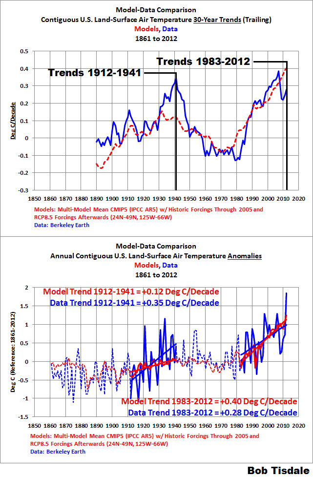
Figure 5

A few things stand out in the top graph of Figure 5. First, the observed 30-year warming rates ending in the late-1930s, early-1940s are comparable to the most recent observed 30-year trends. In other words, there’s nothing unusual about the most recent 30-year warming rates of the surface air temperatures for the contiguous U.S.  Nothing unusual at all.

Second, notice the disparity in the warming rates of the models and data for the 30-year period ending in 1941. According to the consensus of the models, the near-surface air of the contiguous United States should only have warmed at a rate of about 0.12 deg C/decade over that 30-year period…if the warming there was dictated by the forcings that drive the models.  But the data indicate the contiguous U.S. surface air warmed at a rate that was almost 3.5 deg C/decade during the 30-year period ending in 1941…almost 3-times higher than the consensus of the models.  That additional 30-year warming observed in the contiguous United States, above and beyond that shown by the consensus of the models, logically had to come from somewhere.  If it wasn’t due to the forcings that drive the models, then it had to have resulted from natural variability.

Third thing to note about Figure 5:  As noted earlier, the observed warming rates for the 30-year periods ending in 2012 and 1941 are comparable.  But the consensus of the models show, if the warming of the near-surface air of the contiguous United States was dictated by the forcings that drive the models, the warming rate for the 30-year period ending in 2012 should have been noticeably higher than what was observed.  In other words, the data show a noticeably lower warming rate than the models for the most-recent 30-year period.

Fourth: The fact that the models better simulate the warming rates observed during the later warming period is of no value.  The model consensus and data indicate that the surface temperatures of the contiguous United States can warm naturally at rates that are more than 2.5 times higher than shown by the consensus of the models.  This suggests that the model-based predictions of future surface warming for the contiguous U.S. are way too high.

CLOSING

Climate science is a model-based science, inasmuch as climate models are used by the climate science community to speculate about the contributions of manmade greenhouse gases to global warming and climate change and to soothsay about how Earth’s climate might be different in the future.

The climate models used by the Intergovernmental Panel on Climate Change) IPCC cannot properly simulate the surface air temperatures of the contiguous United States over any timeframe from 1861 to present.  Basically, they have no value as tools for use in determining how surface temperatures have impacted temperature-related metrics (snowfall, drought, growing periods, heat waves, cold spells, etc.) or how they may be impacting them presently and may impact them in the future.

As noted a few times in On Global Warming and the Illusion of Control – Part 1, climate models are presently not fit for the purposes for which they were intended.

OTHER POSTS WITH MODEL-DATA COMPARISONS OF ANNUAL TEMPERATURE CYCLES

This is the third post of a series in which we’ve included model-data comparisons of annual cycles in surface temperatures.  The others, by topic, were:

• Near-land surface air temperatures of Greenland
• Sea Surface Temperatures of the Main Development Region of Hurricanes in the North Atlantic